Appearance
Blueback Investigator Quick Guide
Equations
Regressions – simple regression
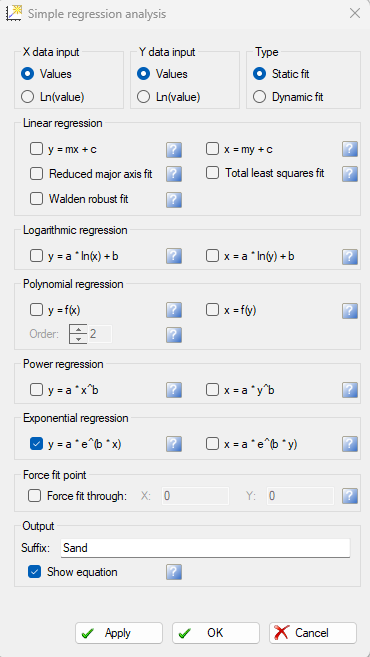
It is easy to run regressions in a 2D cross-plot. Use the ”Add equation” button to access the regressions menu. Select ”Simple regression analysis” to open the regressions menu

Use raw values or natural logarithm on axes data. Select regression type and axis to fit regression
Run multiple regressions in the same cross-plot
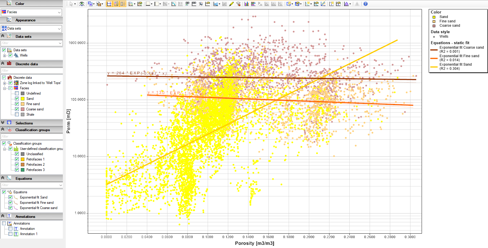
Dynamic fit regressions will interactively update to filtered points
Option to force fit regression
Apply suffix and toggle ”Show equation” to display equation in plot
The regressions cannot be manipulated manually. Use filters to exclude outliers from regression
Regressions – user defined equations
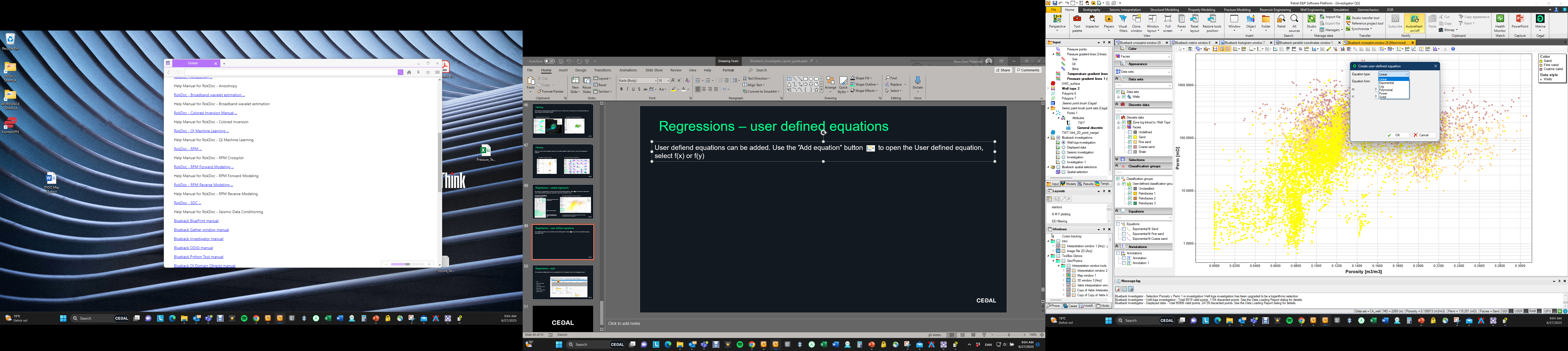
User defined equations can be added. Use the ”Add equation” button to open the User defined equation, select f(x) or f(y) and select equation form
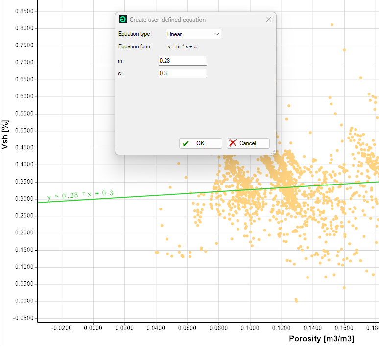
Linear
Exponential
Log
Polynomial
Power
Script (python)
Regressions - style
The regression plotting style can be manipulated from the ”Equations” tab in the investigation panel
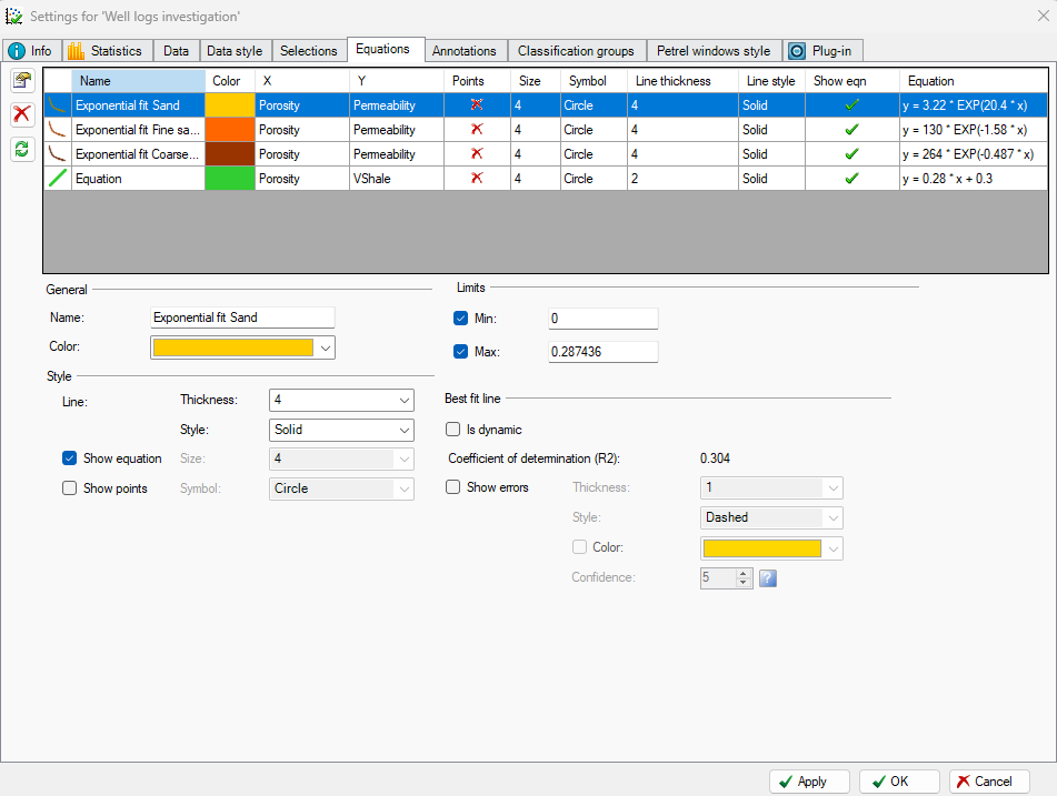
Color
Set min max extent
Thickness
Show equation in plot
Show points
Toggle dynamic status
Show error bars
Manipulate user equations
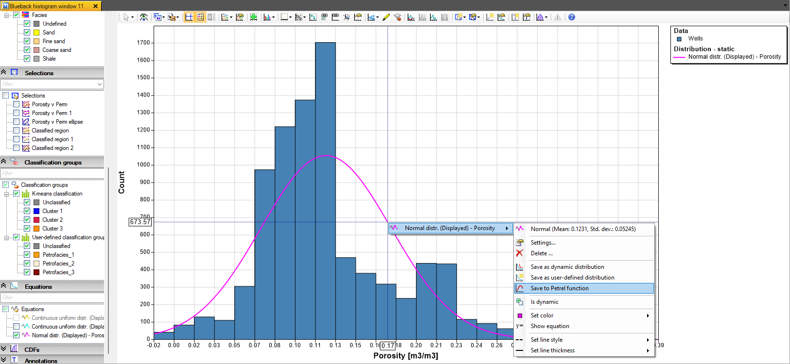
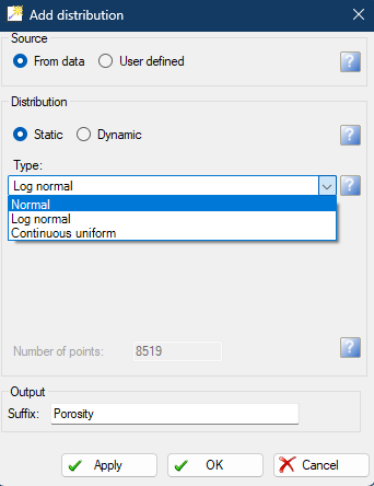
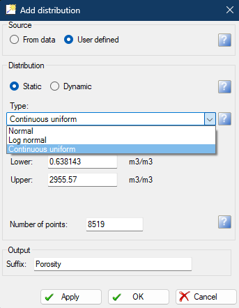
Distributions can be generated from the histogram window. Open the distribution menu by hitting the ”Add distribution” button from the toolbar. Normal, Log normal and Continuous uniform distributions can be generated from the displayed data, or user defined distributions can be generated. The distributions can be saved as Petrel distributions from the RBM context menu. The distributions cannot be manually edited. Use the filter options to specify the data range for the distribution

Discrete classification
Discrete classification of point clusters in cross-plots can be applied manually, using the KMeans algorithm or via Cegal Prizm (external python scripting) The discrete classification workflows work on all supported data types. Examples in this document are performed on well log data
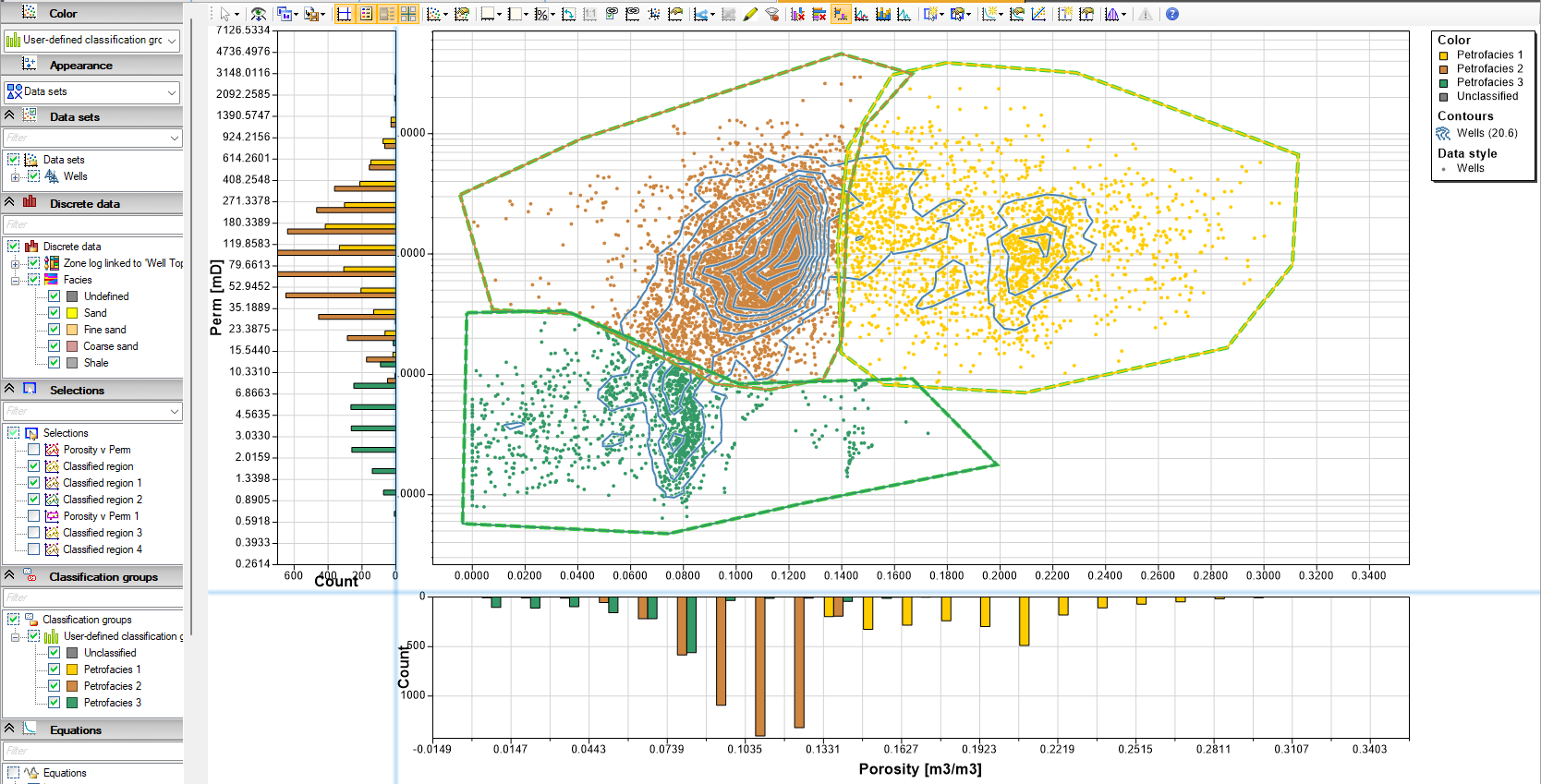
Discrete classification – manual workflow
Define a discrete template in the Classification groups tab
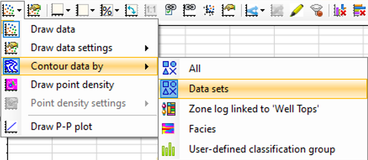
Use histograms, coloring and point density contouring to expose point cluster. Use the ”Classification” regions from the ”Add selection” drop down to circle the clusters
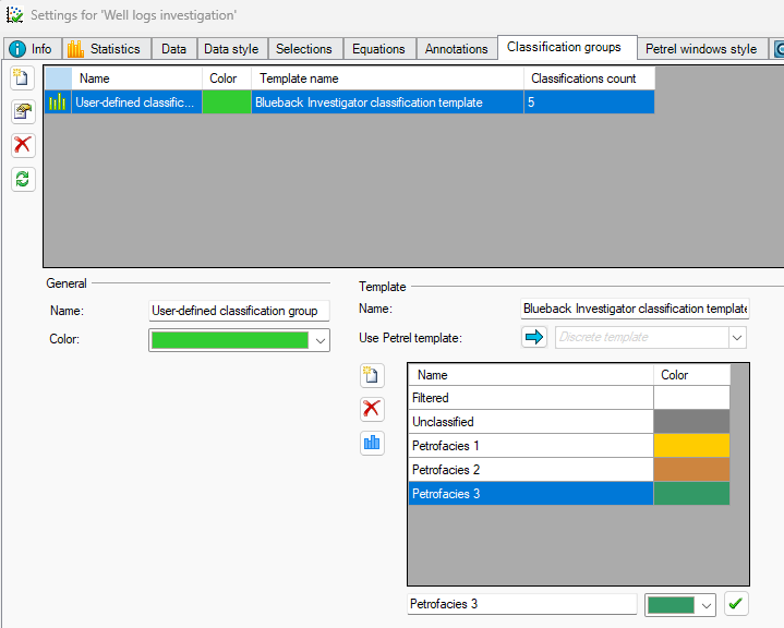
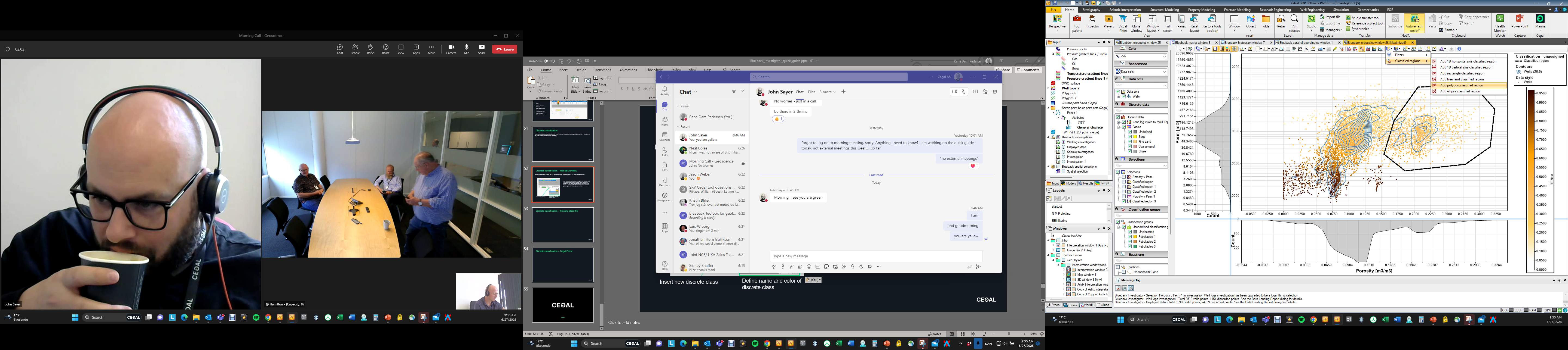
Define name and color of discrete class
Insert new discrete classes
Discrete classification – manual workflow
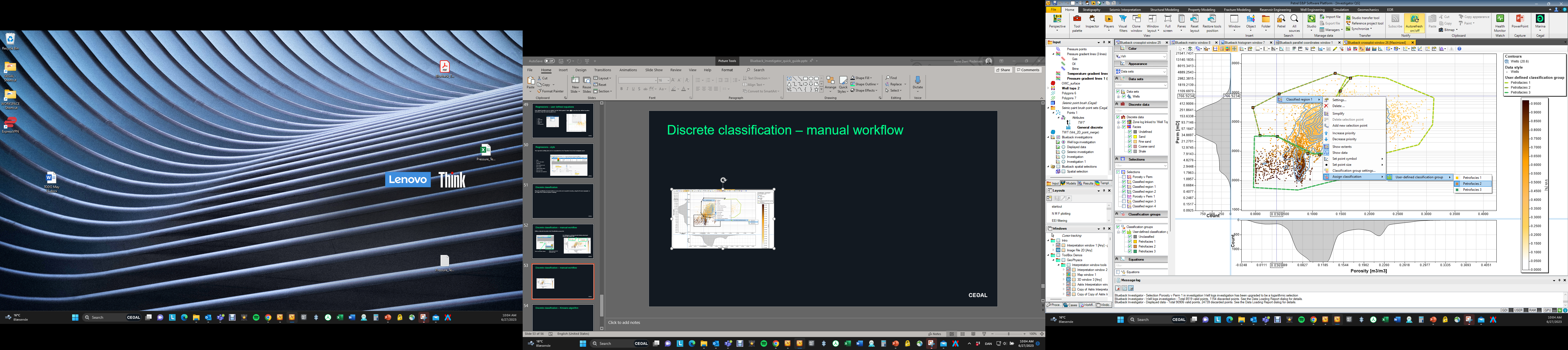
Assign discrete classes defined in the investigation panel to the classification regions
The plotted points can now be colored and filtered by the new classification
RMB on the individual regions ….. select class
Discrete classification – manual classification
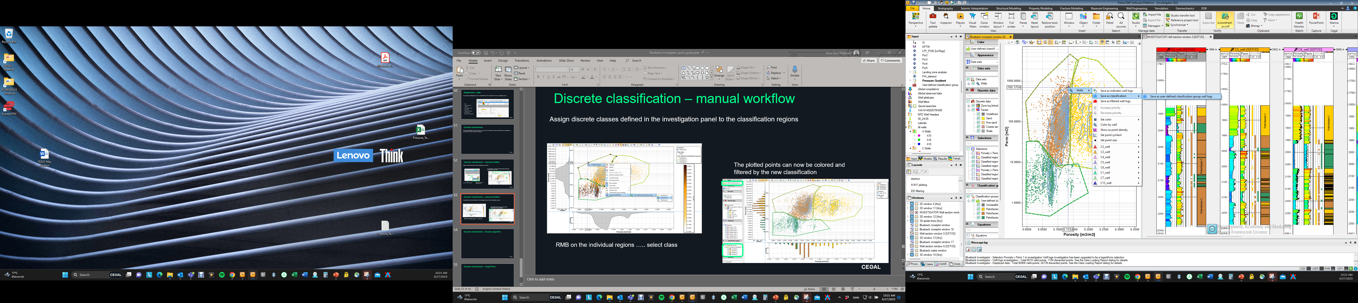
The classification can be saved as a Petrel discrete global well log
RMB on a point in the plot and select ”Save as classification – Save as….” The log is now saved as a new discrete Petrel global well log
Investigation displayed in WSW
Classification saved as discrete well log
Discrete classification – KMeans algorithm
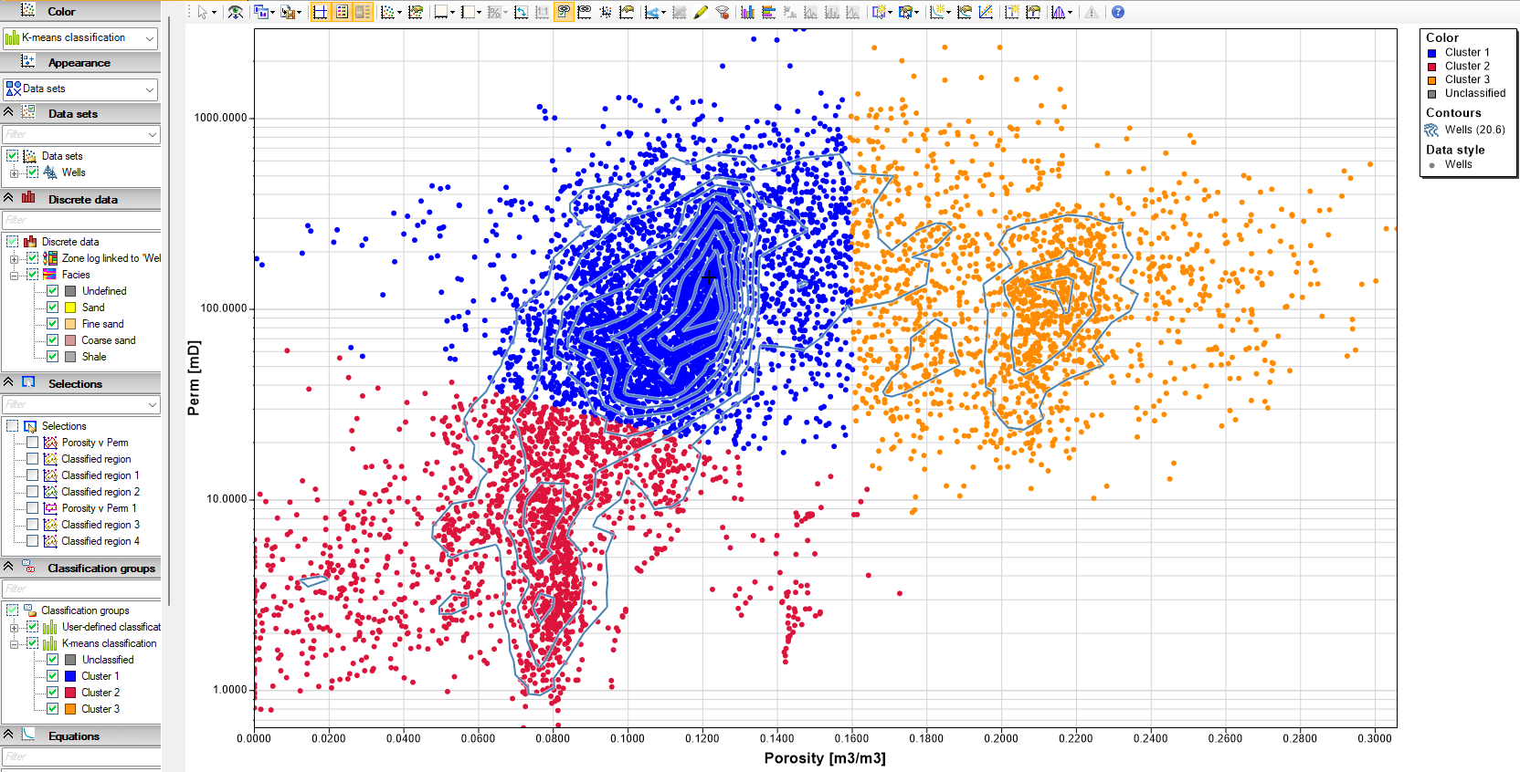
If the point clusters are relatively well defined, the classification can be performed by the KMeans ML algorithm
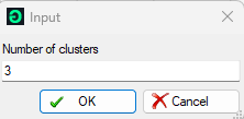
From the “Add equation” button, select “classification equation – Add KMeans classification” Give the number if desired cluster classifications
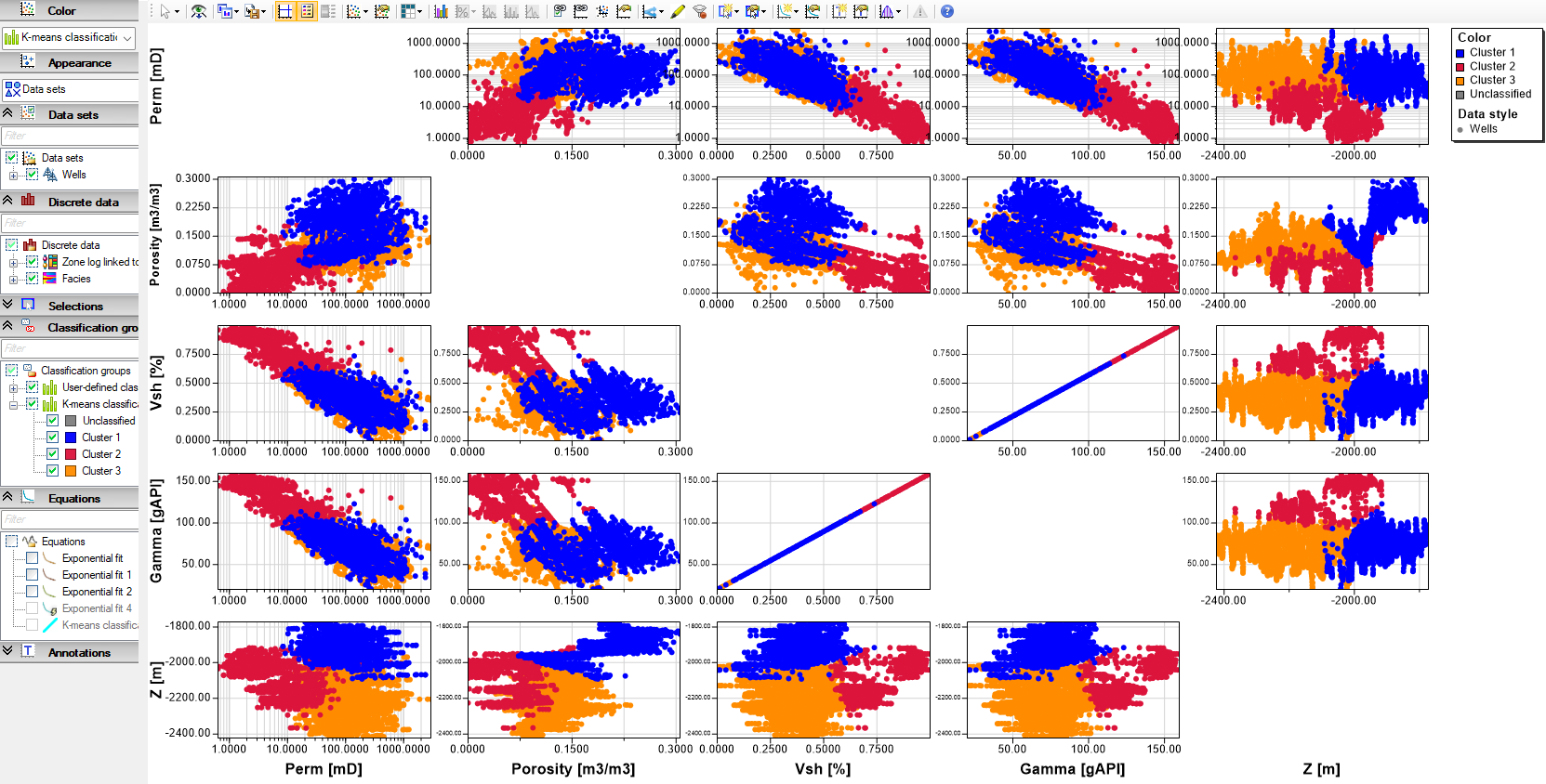

The number of input variables for the KMeans algorithm is defined by the displayed dimensions, in this example 5 input variables
The KMeans classification can be saved as a discrete log in the same way as the manual classification
Discrete classification – Cegal Prizm
ML classification algorithms that are not available in Investigator can be implemented when Blueback Investigator is combined with Cegal Prizm. Build the classification in a Python notebook and implement in the Investigator via Prizm Investigator
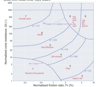
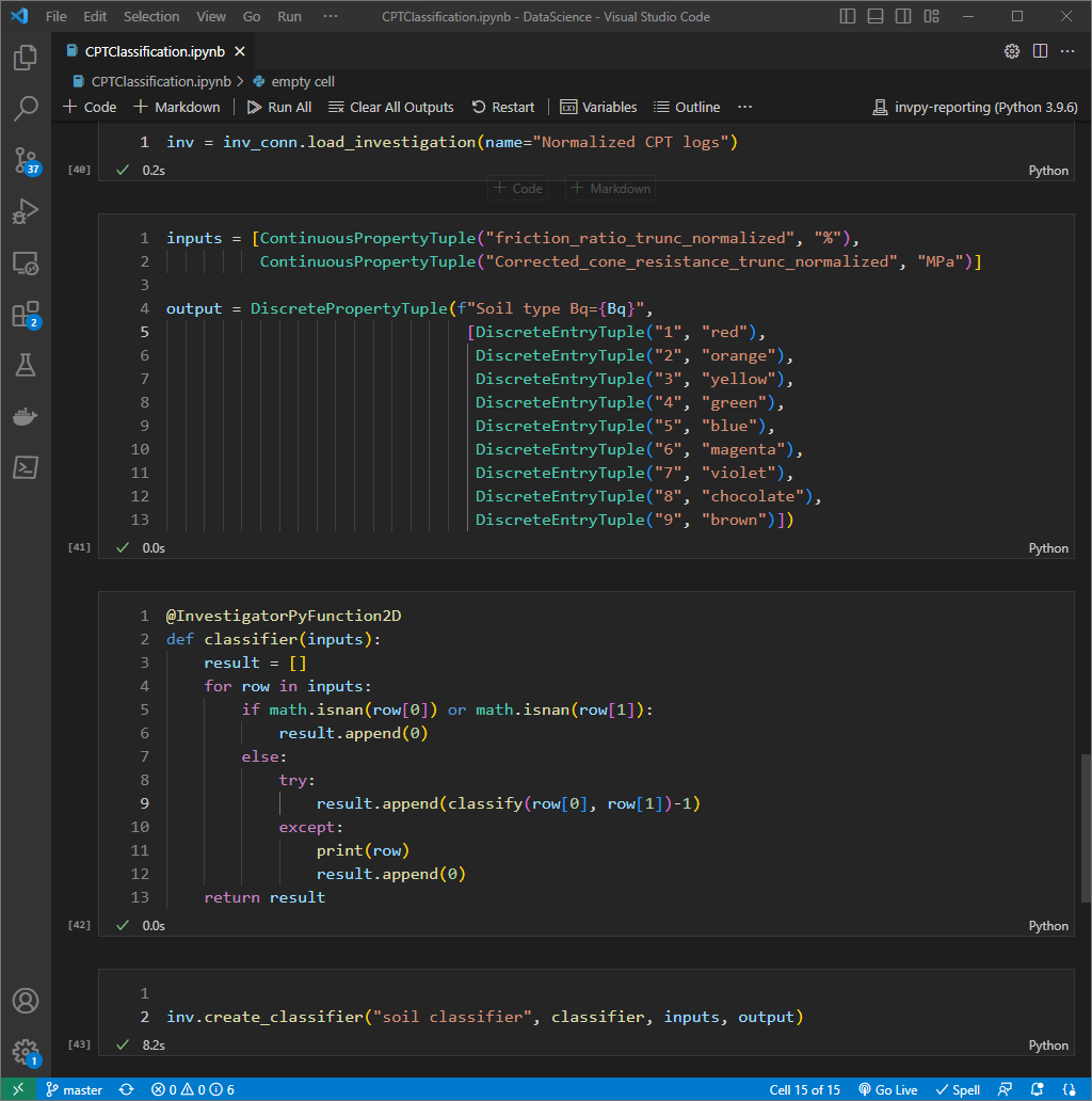
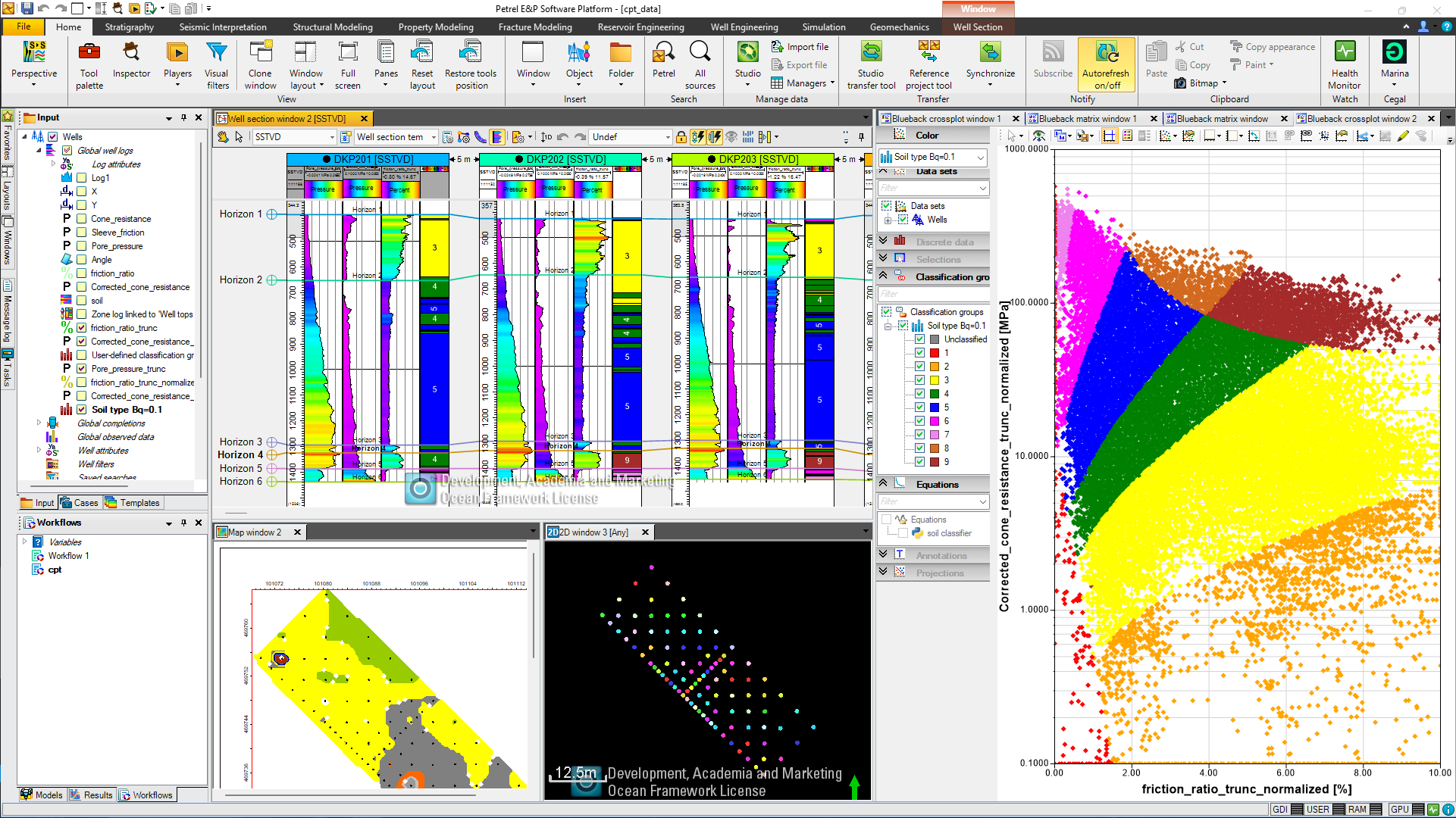
User defined classification built in Python notebook, applied in Petrel via Prizm and then applied on CPT log data via Blueback Investigator