Appearance
[
 {width="6.197916666666667in" height="1.3229166666666667in"}]
[Blueback Investigator 6.0 - User Guide]{.underline}
[Table of Contents]{.underline}
[About Cegal]{.underline}
[Cegal is a tech company writing digital success stories. By delivering leading industry software, world-class consulting, and mission critical cloud solutions, we are shaping the digital future.]
[With 800 employees in eight countries, we are growing to become a leading global technology powerhouse for the energy industry and a contributor to the green transition. The unique combination of IT and geoscience domain expertise puts us in an excellent position to fill the gap between IT and E&P.]
[Our software team provides tools and products for the Petrel platform in order to extend, improve and speed up workflows within geology, geophysics, reservoir engineering and data management. Our strong domain knowledge, both in G&G and software development & commercialization, puts us in a strong position for providing successful software solutions. ]
[Additional software products for the Petrel platform are available from the SLB Ocean Store]{.underline}.
[Visit www.cegal.com]{.underline} for more information.
[Copyright ©2025 Cegal. All rights reserved. ]
[This work contains the confidential and proprietary trade secrets of Cegal and may not be copied or stored in an information retrieval system, transferred, used, distributed, translated or re-transmitted in any form or by any means, electronic or mechanical, in whole or in part, without the express written permission of the copyright owner. ]
[SLB Trademarks & Service Marks ]
[SLB, the SLB logotype, trademarks, trade names or service marks of SLB may not be copied, imitated, or used, in whole or in part, without the express prior written permission of SLB.]
[Introduction]{.underline}
[Introduction]{.underline}
[The Blueback Investigator plugin allows Petrel]{.underline}^[TM]{.underline}^[ users to analyse their data via new plotting functionality that is not currently available within the Petrel histogram or function windows. It has been developed by the Cegal development team using Ocean]{.underline}^[TM]{.underline}^[, the Petrel development kit.]
[Previously this product has been named Blueback Geodata Investigator.]
[Please see relevant release notes for more information. These are available with the installation files or from the support portal]{.underline}.
[History]{.underline}
[Version 1.0 of the Blueback Geodata Investigator adds generic plotting functionality to Petrel.]
[Version 1.1 provides some stability fixes and introduces a few new features. See New for version 1.1]{.underline} for details.
[Version 2.0 adds support for 20 dimensions of data and new visualization windows; the matrix plot and the parallel coordinates plot. See New in version 2.0]{.underline} for details.
[Version 2.1 is a stability release. See New for version 2.1]{.underline} for details.
[Version 2.2 delivers some new features and fixes some stability issues. See New for version 2.2]{.underline} for details.
[Version 3.0 is a major functionality release adding many new features and improving usability. See New for version 3.0]{.underline} for details.
[Version 3.1 is a minor enhancements release which aims to improve integration with Petrel. It also delivers some new features and fixes some stability issues. See New for version 3.1]{.underline} for details.
[Version 4.0 is a major functionality release adding many new features and improving usability. See New for version 4.0]{.underline} for details.
[Version 4.1 is a minor enhancement release which aims to improve the performance when accessing data within Petrel. See New for version 4.1]{.underline} for details.
[Version 4.2 is a minor enhancement release which adds support for Petrel 2016. See New for version 4.2]{.underline} for details.
[Version 4.2.1 is a minor release which adds support for Petrel 2017.]
[Version 5.0 is a major release which significantly improves performance and adds support for new datatypes and various other enhancements/new features. See New for version 5.0]{.underline} for details.
[Version 5.1 is a minor release that adds distribution functionality and two new tools. See New for version 5.1]{.underline} for details.
[Version 5.2 is a minor release that adds new data types and Python integration support. See New for version 5.2]{.underline} for details.
[Version 5.3 is a minor release that adds support for Petrel 2021 . See New for version 5.3]{.underline} for details.
[Version 5.4 is a minor release that adds support for Prizm Investigator. See New for version 5.4]{.underline} for details.
[Version 5.5 is a minor release that adds support for volumetric case data and a new rank-percentile analysis mode alkongside other client requested enhancements. See New for version 5.5]{.underline} for details.
[Version 5.6 is a minor release that adds support for rose diagrams, angular scatterplots and addresses various customer requested usability enhancements. See New for version 5.6]{.underline} for details.
[Ocean]{.underline}
[The Petrel development kit Ocean is central to our development of the Blueback Investigator. With Ocean we have access to the Petrel data model, in addition to tools for making "Petrel-style" user interfaces and workflows. It has proven to be an effective and rapid tool for introducing new technology and functionality to Petrel. Ocean is being developed further to have a broader data type footprint and it still has some limitations to third-party software developers like Cegal. ]
[At Cegal we also undertake larger development projects for generating Petrel plug-in products specific to certain customers. Please get in touch with us on sales.geo@cegal.com]{.underline} if you have any questions or would like to find out more.
[* Ocean and Petrel are trademarks of SLB]
[New for 6.0]{.underline}
[Blueback Investigator 6.0 is a major functionality release that adds the following functionality:]
[Support for Reservoir Engineering data/plots]{.underline}
[·Support for Well observed datasets (see Well observed data]{.underline})
[·Support for Summary Result datasets (see Summary results]{.underline})
[·New Time Series window (see Time series window]{.underline})
[·New timespan classifications (see Timespan classifications]{.underline})
[Minor Enhancements]{.underline}
[·Support for high DPI monitors]
[·New user defined expression equations (see User expression equations]{.underline})
[·New pie chart option (see Pie charts]{.underline})
[·Additional weighted histogram options (see Weighting options]{.underline})
[Prizm Investigator]{.underline}
[·Prizm Environments (see Prizm Environments for Investigator]{.underline})
[·Bundled workflows for Prizm Workflow Runner]{.underline} (see [Bundled workflows]{.underline})
[New for 5.7]{.underline}
[Blueback Investigator 5.7 is a minor functionality release that adds the following functionality:]
[Prizm Investigator]{.underline}
[·Support for Prizm Workflow Runner]
[New for 5.6]{.underline}
[Blueback Investigator 5.6 is a minor functionality release that adds the following functionality:]
[Angular Plots]{.underline}
[·New rose diagram visualization (see Rose diagram]{.underline})
[·New angular scatterplot visualization (see Angular plot]{.underline})
[·Combined linear and angular visualizations (see Angular plots]{.underline})
[Data Selection]{.underline}
[·Improved automatic data selection]
[·Additional region of interest options (see Checkshots]{.underline}, [Well points]{.underline}, [Well tops]{.underline})
[·Reset decimation option (see Model]{.underline}, [Realization folders]{.underline}, [Seismic 2D]{.underline}, [Seismic 2D by vintage]{.underline}, [Seismic 3D]{.underline}, [Simulation cases]{.underline})
[Crossplot window]{.underline}
[·Label scatterplot points option (see Data]{.underline})
[Matrix window]{.underline}
[·Open histogram/crossplot window from viewport (see Opening Linked Windows]{.underline})
[Dimension Axis Settings]{.underline}
[·New symmetrical range option (see Dimensions]{.underline})
[New for 5.5]{.underline}
[Blueback Investigator 5.5 is a minor functionality release that adds the following functionality:]
[Data Loading]{.underline}
[·A new interpolation method for well log data (see Sampling from Dimension (Interpolate other dimensions)]{.underline})
[·Volumetric data type now supported for all users (see Volumetric cases]{.underline})
[Classifications]{.underline}
[·Support for N-dimensional KMeans+ classifications (see Kmeans classification]{.underline})
[Histogram window]{.underline}
[·New Rank-Percentile analysis mode (see Rank-Percentile analysis]{.underline})
[Equation Transformer tool]{.underline}
[·Support for user defined classifications (see Equation transformer tool]{.underline})
[UX Improvements]{.underline}
[·New filtering/groups controls added to statistics table (see Filter/grouping controls]{.underline})
[·Add control for histogram bar labeling (see Histogram]{.underline})
[·Discrete plot ordering (see Discrete plots]{.underline})
[·New plot axis tooltips (see Discrete plots]{.underline})
[New for 5.4]{.underline}
[Blueback Investigator 5.4 is a minor functionality release that adds the following functionality:]
[Prizm Investigator]{.underline}
[·Improved Python support for Blueback Investigator (see .invpy]{.underline})
[UX Improvements]{.underline}
[·Improvements when selecting realization folders and simulation dates (See Realization folders]{.underline})
[Histograms]{.underline}
[·Histograms have been updated to use a common count axis range, where necessary, making discrete plots much more useful and intuitive.]
[New for 5.3]{.underline}
[Blueback Investigator 5.3 is a minor functionality release that adds the following functionality:]
[Petrel 2021]{.underline}
[·Add support for Petrel 2021]
[UX Improvements]{.underline}
[·Add filtering option when selecting realization folders (See Realization folders]{.underline})
[Internal Refactoring]{.underline}
[·A significant amount of refactoring has occured to the product internals. This should have no impact on the user in this release but lays foundations for features in future releases. ]
[New for 5.2]{.underline}
[Blueback Investigator 5.2 is a minor functionality release that adds the following functionality:]
[Supported data types]{.underline}
[·Support added for simulation cases (see Simulation cases]{.underline})
[·Support added for realization folders (see Realization folders]{.underline})
[·Support added for volumetric cases (see Volumetric cases]{.underline})
[Histogram window]{.underline}
[·Support for bar charts (histograms of discrete data) (see Bar charts]{.underline})
[InvestigatorPy (now renamed to Prizm]{.underline}[ Investigator]{.underline})
[·Support for accessing investigation object from Python (see .invpy file]{.underline})
[·Support for saving prediction functions in Python and run these within Petrel Investigations (see Import Python prediction equation]{.underline})
[·Support for saving classification functions in Python and run these within Petrel Investigations (see Import Python classification equation]{.underline}}
[Equations]{.underline}
[·Treat equations as computed dimensions (see Computed dimensions]{.underline})
[Miscellaneous new features/enhancements]{.underline}
[·Data selection improvements (see multi-select]{.underline})
[·Allow user to control what statistics information is drawn in bag plots (see Bag plot]{.underline})
[·Save transformation equations from Principal Component Analysis (see Principal component analysis]{.underline})
[New for 5.1]{.underline}
[Blueback Investigator 5.1 is a minor functionality release that adds the following functionality:]
[Supported data types]{.underline}
[·Support added for Discrete seismic (Subset of existing 3D seismic support)]
[Equations]{.underline}
[·Possible to create and visualize data distributions]
[Miscellaneous new features/enhancements]{.underline}
[·New tool - Data reshaper]
·New tool - [Discrete template generator]
[New for 5.0]{.underline}
[Blueback Investigator 5.0 is a major functionality release that adds the following functionality:]
[Performance]{.underline}
[·All queries/operations are now multi-threaded]
[·Memory usage has been reduced]
[·Much improved support for a large number of datasets (eg. 5000 wells)]
[Supported datatypes]{.underline}
[·Support added for well point logs (see Well points]{.underline})
[·Support added for well top attributes (see Well tops]{.underline})
[·Support added for checkshots (see Checkshots]{.underline})
[·Wells datatype has been renamed to well logs]
[Equations]{.underline}
[·Usability improvements to best fit creation (see Simple regression analysis dialog]{.underline})
[·Support for Ln(V) fits (see Simple regression analysis dialog]{.underline})
[·New linear regressions]
[·Reduced major axis regression]
[·Total least squares regression]
[·Walden robust regression]
[·Display equations as Ln or Log10 (see Ln or Log10 equations]{.underline})
[Usability]{.underline}
[·Create investigation from ribbon (see Petrel UX]{.underline})
[·Display currently selected objects in an Investigator window (see Petrel UX]{.underline})
[Miscellaneous new features/enhancements]{.underline}
[·Data loading report (see Data loading report]{.underline})
[·Unique dimensions]
[The limitation that 2D filters/classifications can only be applied when the dimension templates differ has been resolved. ]
[·Appearance by options (see Appearance of data]{.underline})
[·Support for data overplotting in scatterplots (see Overplot data and decimation]{.underline})
[·Option to control plot decimation in scatterplots (see Overplot data and decimation]{.underline})
[·Logarithmic ticks now forced to be drawn on decades]
[·Option to flip histograms in crossplot window (see Histogram toolbar]{.underline})
[·Option to draw histograms as horizontal bars (see Plot axes]{.underline})
[Removed/deprecated features]{.underline}
[·Individual well log dataset has been removed]
[Use well logs dataset instead. This allows well logs from one or more well to be loaded based on the global well logs. (see Well logs]{.underline})
[·Quick start histogram tool has been deprecated (please contact support]{.underline} if access is still required)
[·Quick start crossplot tool has been deprecated (please contact support]{.underline} if access is still required)
[New for 4.2]{.underline}
[Blueback Investigator 4.2 is a minor functionality release that adds the following functionality:]
[Petrel 2016]{.underline}
[·Adds support for Petrel 2016]
[·Adds support for warm license checkout]
[Miscellaneous new features/enhancements]{.underline}
[·Numeric precision improvements (Dimensions]{.underline})
[Removed features]{.underline}
[·Dynamic point sets have been removed. This was replaced in previous release with the ability to display investigations directly in Petrel windows (Relating conceptual and real world space]{.underline})
[New for 4.1]{.underline}
[Blueback Investigator 4.1 is a minor functionality release that adds the following functionality:]
[Petrel 2015]{.underline}
[·Adds support for Petrel 2015]
[Miscellaneous new features/enhancements]{.underline}
[·Data loading performance improvements]
[·Rebranded to Cegal]
[New for 4.0]{.underline}
[Blueback Investigator 4.0 is a major functionality release that adds the following functionality:]
[Statistics]{.underline}
[·Statistics in all windows (see Statistics]{.underline})
[·Statistics overlays - Box plots and bag plots (see Statistics overlays]{.underline})
[·Principal Component Analysis (see Principal Component Analysis]{.underline})
[·Percentile-Percentile plots (see Percentile-Percentile plots]{.underline})
[Visualization]{.underline}
[·Multi-dimension histograms (see Multi-dimension histograms]{.underline})
[·Discrete plots (see Discrete plots]{.underline})
[Equations]{.underline}
[·Calculated dimensions (see Calculated dimensions]{.underline})
[·Equation transformer tool (see Equation transformer tool]{.underline})
[·Multi-linear regression (see Multi-linear regression]{.underline})
[·Bayesian classification (see Bayesian classification]{.underline})
[Selections]{.underline}
[·2D ellipse filter (see Ellipse selection method]{.underline})
[·3D box filter (see Box selection method]{.underline})
[·3D ellipsoid filter (see Ellipsoid selection method]{.underline})
[·Use Blueback Spatial Selector as a filter (see Blueback Spatial selections as filters]{.underline})
[·Auto-classification using Kmeans clustering (see Auto-classification]{.underline})
[Miscellaneous new features/enhancements]{.underline}
[·Minimum viewport size (see Window settings dialog]{.underline})
[New for 3.1]{.underline}
[Blueback Geodata Investigator 3.1 is a minor enhancement release that adds the following functionality:]
[Blueback spatial selector ]{.underline}[(see Blueback spatial selector help for more information)]
[·Visualize and manipulate spatial selector in well section window]
[·Undo/redo support]
[·Expand to include selected Petrel object(s).]
[·Create spatial selector enclosing selected object(s)]
[Visualization]{.underline}
[·Display investigation in the Petrel well section window (see Petrel well section window]{.underline})
[·Display investigation in the Petrel seismic windows (see Petrel seismic windows]{.underline})
[·Display investigation in the Petrel map window (see Petrel map window]{.underline})
[·Link visible objects between windows (see Link visible objects]{.underline})
[Miscellaneous new features/enhancements]{.underline}
[·Legend alignment options (see Legend alignment]{.underline})
[·Copy/paste window support]
[·Window settings (see Window settings]{.underline})
[New for 3.0]{.underline}
[Blueback Geodata Investigator 3.0 is a major functionality release that adds the following functionality:]
[Blueback spatial selector]{.underline}
[·What is the Blueback spatial selector? (see Blueback spatial selector]{.underline})
[·Integration with Blueback Investigator (see Using spatial selections within Blueback Investigator]{.underline})
[·Create investigation from spatial selection (see Create investigation from spatial selection]{.underline})
[Tools]{.underline}
[·Quick start histogram tool (see Quick start histogram tool]{.underline})
[·Quick start crossplot tool (see Quick start crossplot tool]{.underline})
[Workflow support]{.underline}
[·Basic workflow support (see Worksteps]{.underline})
[Visualization]{.underline}
[·3D plot window (see 3D plot]{.underline})
[·Display investigation in the Petrel 3D window (see Petrel 3D window]{.underline})
[·Data highlighting (see Data highlighting]{.underline})
[Usability improvements]{.underline}
[·Data selection changes (see Data selection]{.underline})
[·New window control panel (see Window control panel]{.underline})
[·A new Petrel toolbar has been added providing easier access to Blueback Investigator menu options]
[Miscellaneous new features/enhancements]{.underline}
[·Relative percentage axis on histograms (see Histogram axis]{.underline})
[·Logarithmic selections are now applied in logarithmic space (see Selections]{.underline})
[·Equations in Matrix window (see Matrix]{.underline} window)
[·Limit equation to range (see Equations tab]{.underline})
[·Copy dataset (see Datasets]{.underline})
[·Optional histograms (see Crossplot]{.underline} and [Matrix]{.underline} windows)
[·Improved support for missing data (see Missing values]{.underline})
[·Add no interpolation option when loading well data (see Well logs]{.underline})
[·Add option to support missing cells in table data (see Table data]{.underline} and [Import table data]{.underline})
[Petrel UX - 2014 only]{.underline}
[·Support for the Petrel UX (see Petrel UX - 2014 only]{.underline})
[New for 2.2]{.underline}
[Blueback Geodata Investigator 2.2 is a minor enhancement release that adds the following functionality:]
[·Allow continuous data selection by template units rather than template (see Continuous data]{.underline})
[·Allow user to specify domain and step interval when interpolating well data (see Well logs]{.underline})
[·Allow user to create selections by digitizing a polygon (see Polygon selection]{.underline})
[·Allow user to add/remove control points from polygon and freehand selections (see Freehand selection method]{.underline} and [Polygon selection method]{.underline})
[·Allow user to simplify the number of control points forming a polygon and freehand selection (see Freehand selection method]{.underline} and [Polygon selection method]{.underline})
[·Allow user to control dataset priority (see Dataset priority]{.underline})
[·Add x=f(y) equations (see Equations]{.underline})
[·Allow equations to be displayed in swapped axis space (see Equations]{.underline})
[·Allow discrete data in table data (see Table data]{.underline})
[·Allow spatial data in table data (see Table data]{.underline})
[New for 2.1]{.underline}
[Blueback Geodata Investigator 2.1 is a patch release that fixes the following issues:]
[·Stability fixes for display of Rock Physics models]
[·Blueback Investigator classifications --fixes to project save and opening of projects with classifications]
[·Data loading performance improvements]
[New for 2.0]{.underline}
[Blueback Geodata Investigator 2.0 is a major functionality release that adds the following functionality:]
[20 dimensional support]{.underline}
[Support for up to 20 dimensions (Discrete + Continuous)]
[Matrix window]
[New window specialized to display many dimensions at once]
[Parallel coordinates window]{.underline}
[Easy to spot correlations between dimensions]
[General Window usability improvements]
[Context menu support in numerous location]
[Copy enhanced metafile to clipboard]
[Cross hair]
[Cross/scatter-plot windows]
[Contour data option]
[Pick messages to point density plots]
[Ruler tool for spatial plots]
[Support for Rock physics models created in Blueback Rock physics]
[Display Petrel functions]
[Draw Petrel functions and apply spline]
[Export contours to 2D PDF (Usable in Blueback Rock physics)]
[Export raw crossplot object]
[Point densities now honor axis settings]
[Editable best fit lines]
[Dynamic equations]
[Histogram window]{.underline}
[Save histogram line as Petrel function]
[Save CDF as Petrel function]
[Allow user defined CDF percentiles]
[Display weighted histograms]
[Display median, standard deviation and variance in statistics]
[Improved color scale management]{.underline}
[New data selection dialog]
[Support for more dimensions being added]
[Drop down control boxes inside of data selection tables]
[Drop down boxes performs up to 10X faster than before]
[Classification groups tab is added]
[Appearance is renamed "Data style"]
[Spatial dimensions. X,Y, Time, Depth available as built in dimensions]
[Load upscaled cells only for model data]
[Axes tab integrated into new Data->Dimension tab. Can now control axes per window or per investigation]
[Point set support]
[Classification workflow]
[Retired functionality]
[Simple selection or "Quick look" has been retired from Blueback Investigator 2.0. The only way to plot data now is from the investigation.]
[Changes to terminology]{.underline}
[Restrictions have been renamed to selections. See Selections for more details.]
[New for 1.1]{.underline}
[Blueback Geodata Investigator 1.1 has the following new features:]
[Investigation improvements ]{.underline}
- [Easier to tune the size of the investigation]
- [Performance improvements]{.underline}
[Rendering improvements]
[Memory usage is reduced ]
- [Export options ]{.underline}
[Export to spreadsheet ]
[Save investigation as point set ]
- [How does my data translate from plot space into real world space? ]{.underline}
[Toggle dynamic point set - display all investigation data into a point set]
[Create indicator objects - display the selected or visible data as a Boolean volume, log or a property.]
- [Other improvements ]{.underline}
[Improved 2D seismic handling ]
[Well data tops filtering in the investigation ]
[Point density display update ]
[Best fit line update ]
[Release strategy and development plans]{.underline}
[Our release strategy is aggressive and we are investing considerable resources in providing an up-to-date tool with top class support. ]
[All our development is based on input and suggestions from Petrel users around the world and we encourage you all to forward your ideas to support.geo@cegal.com]{.underline} or visit the [support portal]{.underline} to submit your ideas.
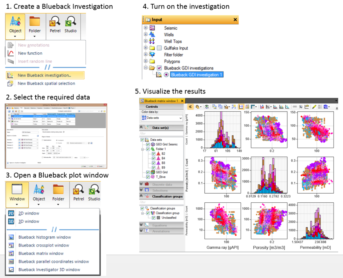
[This section provides an overview of how to get started with Blueback Investigator on the different Petrel platforms. The behavior is different on the different Petrel versions due to the Petrel UX features in Petrel 2014 onwards.]
[See the section Data selection]{.underline} for more details.
[Getting started]{.underline}
[
 {width="6.197916666666667in" height="5.010416666666667in"}]
[Example uses of Blueback Investigator]{.underline}
[Please visit the Cegal Media Center]{.underline} for video examples on how to use Blueback Investigator.
[Concepts and terminology]{.underline}
[This section describes the different concepts and terminology used in the Blueback Investigator.]
[The Blueback Investigator separates data selection from data visualization. ]
[In normal Petrel data is generally turned on and then visualized in the windows. In Blueback Investigator the user needs to spend some time up front before visualizing data. The key to the separation of data selection and visibility is the Blueback investigation]{.underline}.
[Users select the data they might want to investigate or analyze further; this data is then loaded in such a way that the user can visualize this data using different views in multiple windows without the need to reselect the data each time. This allows the user full freedom to select which data is displayed in each view and also the ability to change the data being investigated at any time, or to add new data to the investigation. All loaded data has to belong to a predefined dimension]{.underline}.
[Datatype, Dataset and Dimension]{.underline}
[The following definitions are used throughout this user guide:]
[·A ]{.underline}[datatype]{.underline}[ is the Petrel data object that is used as input to the Blueback investigation.]
[·The table data type is a special data type in Blueback Investigator that is not a Petrel data object. This object allows the user to set up a spreadsheet with data values, forming a ]{.underline}[customized datatype]{.underline}[.]
[·A ]{.underline}[dataset]{.underline}[ is a combination of same data types put together in a collection, or a single individual data type used standalone.]
[·A ]{.underline}[dimension]{.underline}[ is defined by a Petrel template. A dimension is either continuous]{.underline} (
 {width="0.14583333333333334in" height="0.14583333333333334in"}) or [discrete]{.underline} (
 {width="0.14583333333333334in" height="0.13541666666666666in"}).
[·]{.underline}[Spatial dimensions]{.underline}[ are built in special continuous dimensions, enabling spatial data analysis in Blueback Investigator. (X, Y, Time and Depth)]
[·In Blueback Investigator ]{.underline}[spatial]{.underline}[ and ]{.underline}[normal]{.underline}[ dimensions are used in combination with datasets to create the Blueback investigation.]
[·A ]{.underline}[sample]{.underline}[ describes the collection of dimension values that are co-located within a dataset. For example, an IJK cell within a model is used to co-locate all the different dimension values together to form a sample.]
[·A ]{.underline}[computed dimension]{.underline}[ is defined by either a prediction or classification equation. The result of calculating the equation on every sample will be available within the investigation and can be used like any other continuous or discrete dimension.]
[Dimensions]{.underline}
[The following dimension types are supported:]
[Continuous dimensions]{.underline}
[In Petrel continuous templates (
{width="0.14583333333333334in" height="0.14583333333333334in"}) are used along with continuous data. Typically this can be well logs such as Vp, Vs, Porosity etc. In Blueback Investigator templates form Dimensions]{.underline}.[By default, Blueback Investigator limits the selection of continuous data within a dataset to those objects which have the same template as the chosen dimension. This can be quite restrictive to the user. ]
[For example, if the user wishes to investigate well log permeability data and permeabilityI, permeabilityJ and permeabilityK model properties then the user would need to re-assign these objects to the same template.]
[Blueback Investigator provides a button in the continuous data selection control to allow the user to swap between selection of objects based on template or unit category.]
[In template selection, the user can choose from the tree any object which has exactly the same template as the dimension template]
[In unit category selection, the user can choose from the tree any object which uses the same unit category as the dimension template]
[ ]
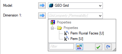
[For example, if the user selects data using the permeability template for model data they would have the following options]
[
 {width="4.114583333333333in" height="1.84375in"}]
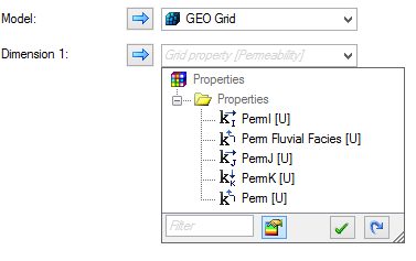
[If the user clicks the
 {width="0.23958333333333334in" height="0.21875in"} button then they are selecting by the permeability unit category and they would have the following options ]
[
 {width="3.9270833333333335in" height="2.46875in"}]
[The user can return to template based selection by clicking the
 {width="0.23958333333333334in" height="0.21875in"} button.]
[Blueback Investigator distinguishes between defining continuous data and discrete data in the set up of the investigation. This is because they are used in slightly different ways in the product. See Coloring data]{.underline} for more information on how to color data in plots.
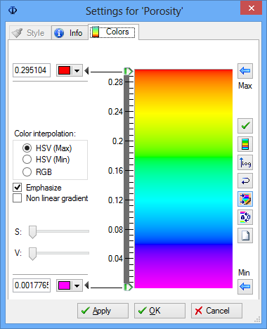
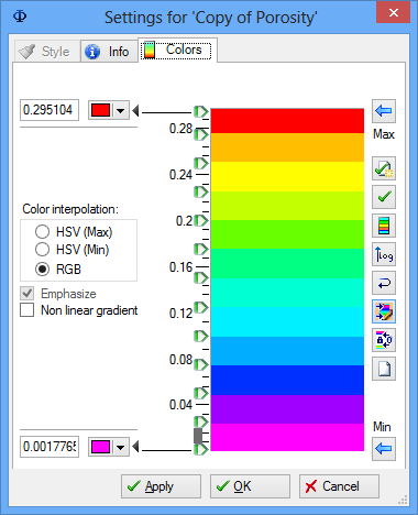
[A continuous template can get a "discrete appearance" by adding fixed color intervals to the color table.]
[
 {width="3.9583333333333335in" height="4.875in"}
 {width="3.9583333333333335in" height="4.875in"}]
[Spatial dimensions]{.underline}
[Spatial dimensions allow X, Y, Time and Depth information to be included in the investigation. The values for these dimensions will be determined from the selected Petrel domain objects in each dataset.]
[Investigations must contain spatial dimensions if the investigation is to be rendered in the supported Petrel windows and/or be used with the Blueback Spatial Selector.]
[Discrete dimensions]{.underline}
[In Petrel discrete color tables are used to assign colors to discrete data, such as facies, fluid information, lithology etc. The discrete color tables are a part of the the discrete templates found in the Templates explorer in Petrel.]
[Discrete (
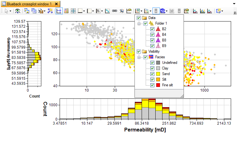
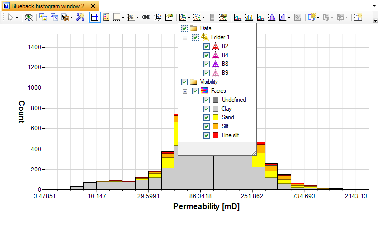
{width="0.14583333333333334in" height="0.13541666666666666in"}) template data (e.g. facies) can be used to color the plot data in all plot windows. ][Data will be colored according to the corresponding template colors as set when the data is added to the plot i.e. updating the colors via the template settings dialog will not update the colors in the plot. ]
[Discrete data can also be used as a visibility filter so, for example, data belonging to a particular facies or group of facies can be toggled on/off allowing the user to focus on data of particular interest.]
[
 {width="6.197916666666667in" height="3.71875in"}]
[
 {width="6.197916666666667in" height="3.71875in"}]
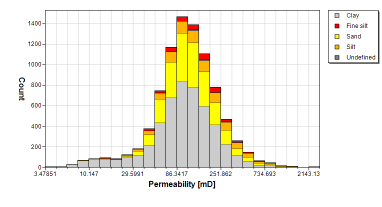
[The window legend displays the discrete color table:]
[
 {width="6.197916666666667in" height="3.3541666666666665in"}]
[Computed dimensions]{.underline}
[A computed dimension can be defined by either a prediction or classification equation. The result of calculating the equation on every sample in the investigation will be available within the investigation and can be used like any other continuous or discrete dimension. Computed dimensions are not shown in the data selection dialog.]
[To create a computed dimension from an equation, the user should set the equation to ]{.underline}[Include as dimension]{.underline}[ (
 {width="0.16666666666666666in" height="0.16666666666666666in"}) using the equation context menu. After the equation has been applied, it will appear everywhere a continuous or discrete dimension is available for selection.]
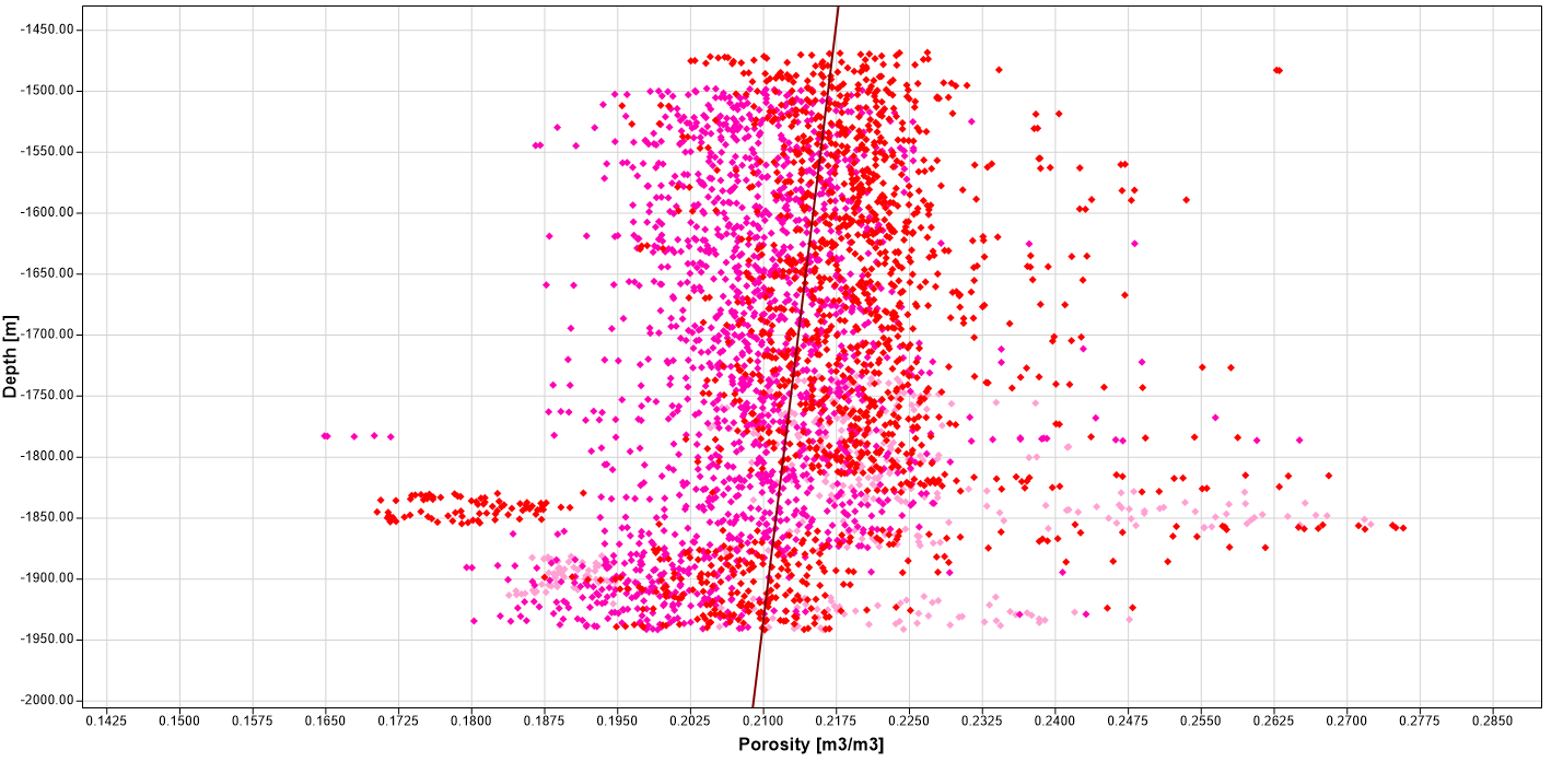
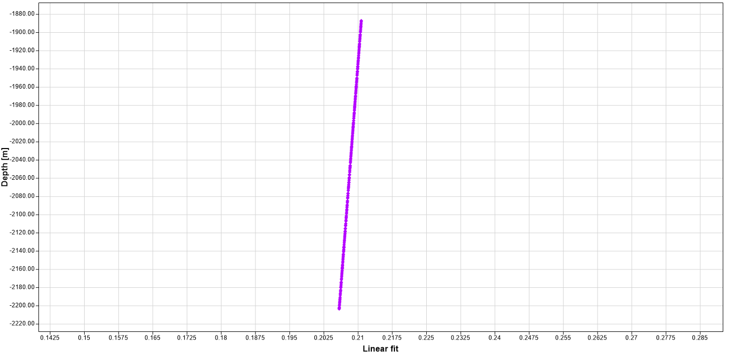
[For example, a simple linear regression can be calculated to determine a relationship between a property and depth.]
[
 {width="6.197916666666667in" height="3.0208333333333335in"}]
[This equation can then be used to predict values in a different well.]
[
 {width="6.197916666666667in" height="3.0208333333333335in"}]
[Blueback investigation]{.underline}
[A Blueback investigation is a grouping of data that the user wishes to analyze and sits at the heart of the Blueback Investigator functionality.]
[A user sets up a Blueback investigation by selecting the data they wish to investigate (see Data selection]{.underline}). This investigation can then be used to provide the source data for a variety of plots. It also acts as a central repository for any selections, equations and annotations created in any plot based on the Blueback investigation, allowing these objects to be shared between plots based around the same Blueback investigation.
[A Blueback investigation can contain up to 20 dimensions]{.underline}[ ]{.underline}[(Total of all continuous (
 {width="0.14583333333333334in" height="0.14583333333333334in"}) and discrete (
 {width="0.14583333333333334in" height="0.13541666666666666in"}) dimensions combined, including spatial dimensions). ]
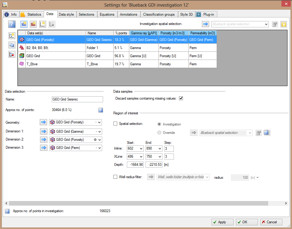
[The definition of the investigation can be edited using the buttons to add the required datasets (
 {width="0.22916666666666666in" height="0.22916666666666666in"}), continuous (
 {width="0.23958333333333334in" height="0.23958333333333334in"}), discrete (
 {width="0.23958333333333334in" height="0.23958333333333334in"}) and spatial (
 {width="0.20833333333333334in" height="0.21875in"}) dimensions. The datasets can then be defined by selecting the row in the table and using the controls that appear below the table. To edit the dimensions, the column header should be selected and can be edited using the controls that appear below the table.]
[E.g: Add many wells (]{.underline}[Data type]{.underline}[) to investigation 1 called "Development wells" (]{.underline}[Dataset]{.underline}[) and investigate relationships between Permeability, Gamma ray and Porosity (]{.underline}[Dimensions]{.underline}[).]
[
 {width="6.197916666666667in" height="4.864583333333333in"}]
[Share data between windows]{.underline}
[A single Blueback investigation can act as the source data for any number of plots. ]
[For example, with templates defined as porosity, permeability and gamma ray the user could plot:]
[a porosity histogram]
[a gamma ray vs permeability crossplot]
[a porosity vs permeability crossplot]
[a parallel coordinates plot with all the data in the Blueback investigation]
[a matrix plot with all the data in the Blueback investigation]
[all based on exactly the same data. ]
[This way a selection applied to one of the plots can be displayed in any of the other plots and similarly for equations and annotations.]
[Supported data types]{.underline}
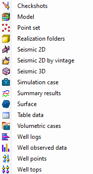
[A Blueback investigation allows the user to select data from the following ]{.underline}[data types]{.underline}[:]
[
 {width="1.9583333333333333in" height="3.65625in"}]
[All of these ]{.underline}[data types]{.underline}[ may be selected within a single investigation so that model properties and well logs, for example, can be compared and analyzed.]
[Table data]{.underline}
[Table data enables the user to load arbitrary data into a Blueback investigation so the user is not limited to data objects that have been made specifically available to the Blueback Investigator (e.g. well logs, model properties etc).]
[The user can specify table data for all dimensions in the investigation - continuous, spatial and discrete. ]
[Continuous and spatial data will be interpreted as numeric values and the user can specify the units in which the table is supplied. ]
[Discrete data is interpreted as strings and only ]{.underline}[tag]{.underline}[ samples correctly if the string specified matches a string in the discrete template color table. The string matching is case insensitive. Any samples that could not be matches will tag the sample as ]{.underline}[undefined]{.underline}[. ]
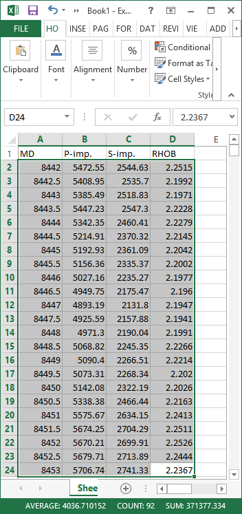
[Values may be entered manually or via a cut & paste option, allowing data to be easily copied from other applications, e.g. Excel, or from the spreadsheet option available for many Petrel data objects.]
[
 {width="3.6666666666666665in" height="7.78125in"}]
[Set up the correct dimensions in the same order as in the excel spreadsheet]{.underline}
[
 {width="6.197916666666667in" height="4.489583333333333in"}]
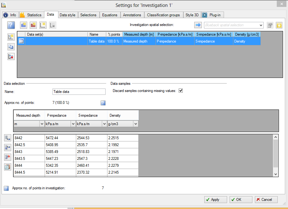
[Use the copy from button to paste into the new investigation]
[The units of the table data values are easily set via the combo boxes at the top of each column. These units have no effect on other options in Petrel i.e. they do not alter projects units or the units displayed on Blueback Investigator plots. They simply specify the units of the entered value, e.g. m/s for P-impedance in the example above so the first value is 5472.55 kPa.s/m. When plotted in a Blueback Investigator plot window these values will automatically be unit converted into the chosen display units.]
[Dataset priority]{.underline}
[The user can control the priority assigned to each ]{.underline}[dataset]{.underline}[ using the Data style]{.underline} tab of the investigation settings dialog.
[Blueback Investigator processes the ]{.underline}[datasets]{.underline}[ in priority order. This means that the first ]{.underline}[dataset]{.underline}[ in the table will be processed first and the ]{.underline}[dataset]{.underline}[ at the bottom of the table will be processed last.]
[This is particularly useful if many ]{.underline}[datasets]{.underline}[ have samples at exactly the same location. Blueback Investigator displays data in reverse priority order, meaning that the samples for the highest priority ]{.underline}[dataset]{.underline}[ will be displayed on top of all the other samples.]
[Data visibility]{.underline}
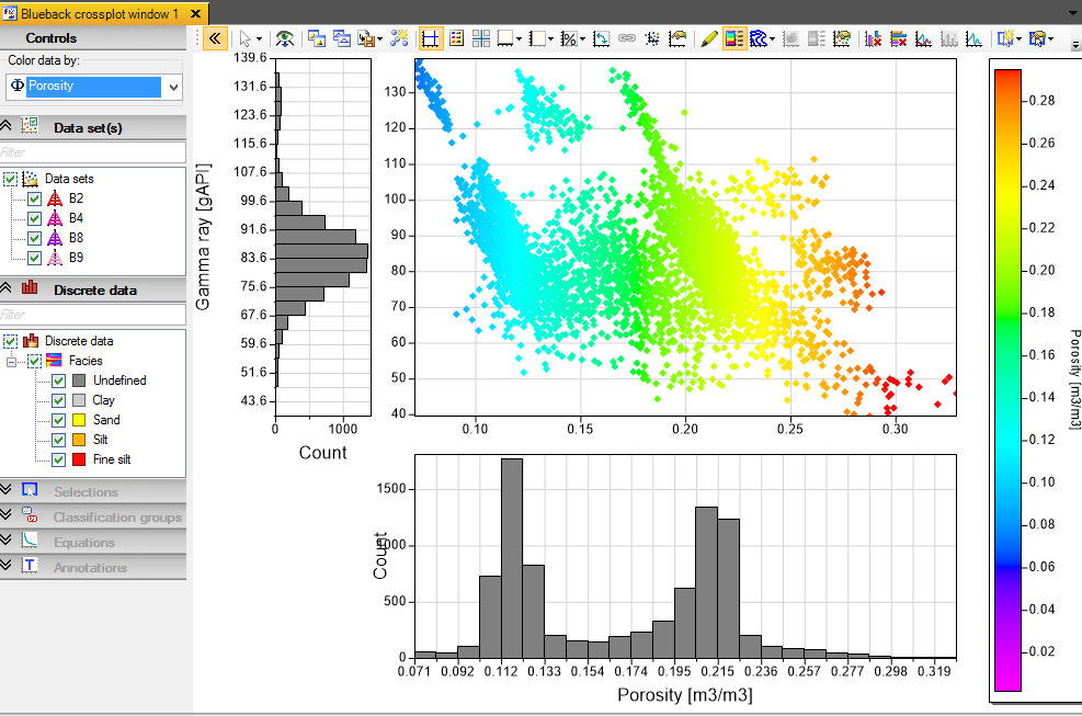
[The Blueback Investigator has options to allow the user to control which data is visualized for certain types of data. In addition to being able to toggle on/off the display of individual discrete data values (e.g. individual facies) users can also control the visibility of data types, e.g. individual wells, model segments & zones etc.]
[
 {width="6.197916666666667in" height="4.09375in"}]
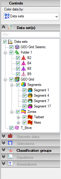
[For models adding any ]{.underline}[segment]{.underline}[ and/or ]{.underline}[zone]{.underline}[ regions of interest exposes new filtering options in the data visibility options.]
[
 {width="2.1354166666666665in" height="6.229166666666667in"}]
[Coloring of data]{.underline}
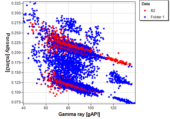
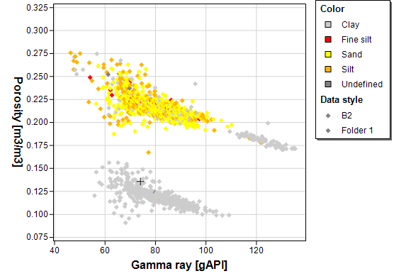
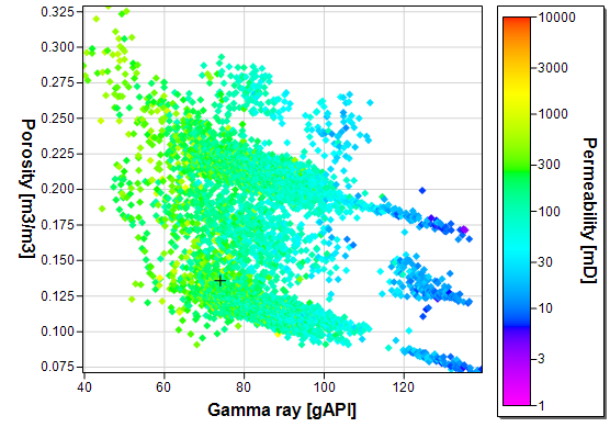
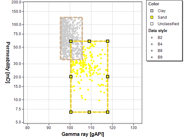
[The Blueback Investigator allows plotted points to be colored by:]
[Color by dataset]{.underline}
[
 {width="5.791666666666667in" height="4.052083333333333in"}]
[Color by discrete data]{.underline}
[
 {width="5.791666666666667in" height="4.052083333333333in"}]
[Color by continuous data]{.underline}
[
 {width="5.791666666666667in" height="4.052083333333333in"}]{.underline}
[Color by classification]{.underline}
[
 {width="6.135416666666667in" height="4.65625in"}]
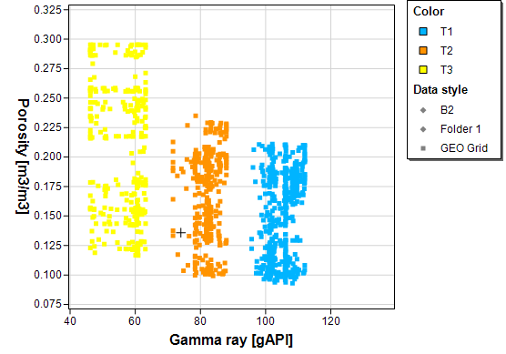
[Color by zone/segment (model properties)]
[
 {width="5.791666666666667in" height="4.052083333333333in"}]
[Color handling in plots]{.underline}
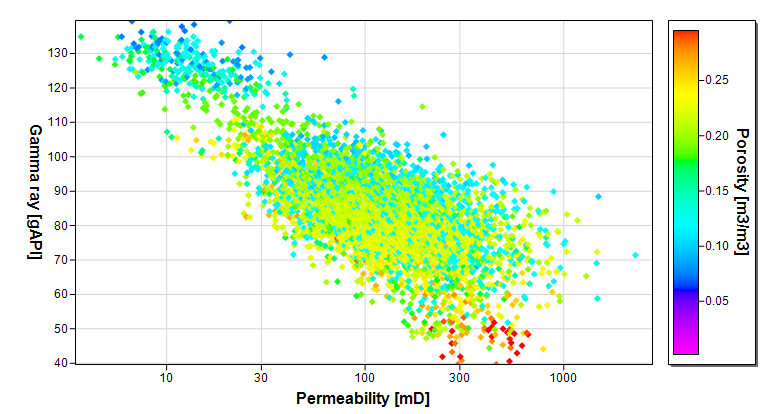
[Blueback Investigator utilizes the colors from the Petrel global template when coloring points in the plot windows and when coloring bars in the histogram window.]
[
 {width="6.197916666666667in" height="3.3541666666666665in"}]
[Permeability plotted against Gamma ray, colored by Porosity]{.underline}
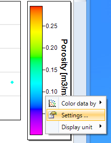
[The color tables used in the Color by]{.underline} feature can be accessed by right clicking the points color scale legend:
[
 {width="2.3333333333333335in" height="3.0208333333333335in"}]
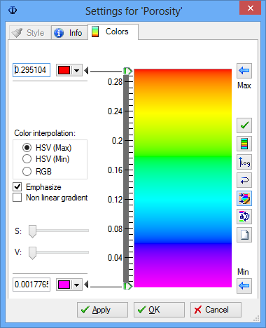
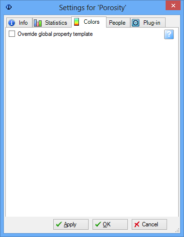
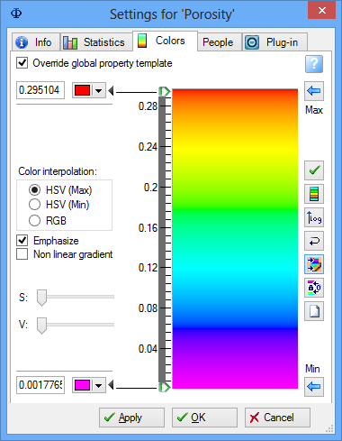
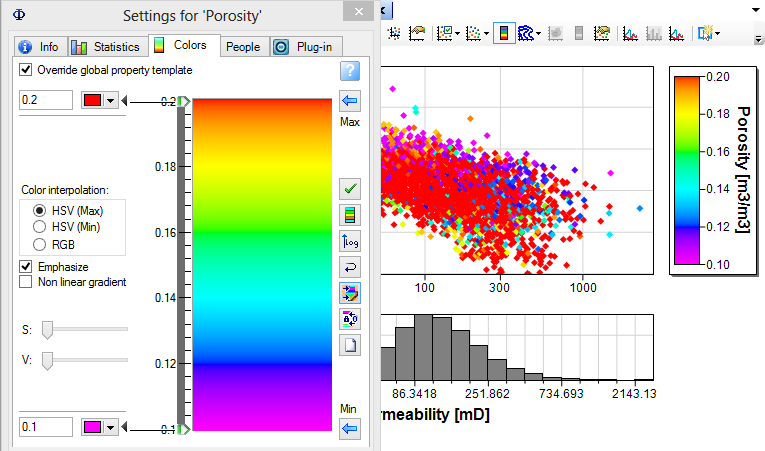
[By default Blueback Investigator uses the global color table from the Global Petrel template. This setting can be overridden inside of the Color table that is exposed inside of Blueback Investigator.]
[
 {width="3.9583333333333335in" height="5.104166666666667in"}
 {width="3.9583333333333335in" height="5.09375in"}
 {width="3.9583333333333335in" height="5.09375in"}]
[Global color table, Global color table as seen in Blueback Investigator and the overridden Color table inside of Blueback Investigator]{.underline}
[Changing the values on the overridden values have immediate effect in the plot:]
[
 {width="6.197916666666667in" height="3.6458333333333335in"}]
[Appearance of data]{.underline}
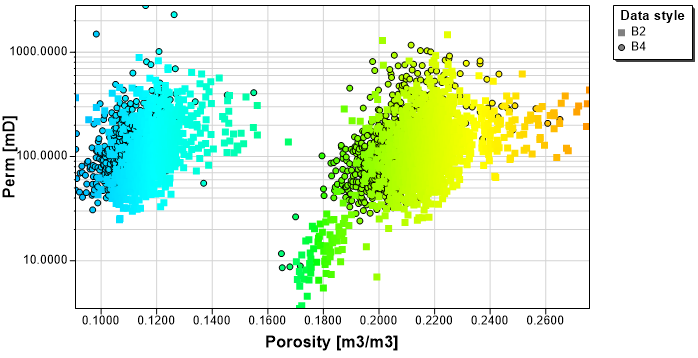
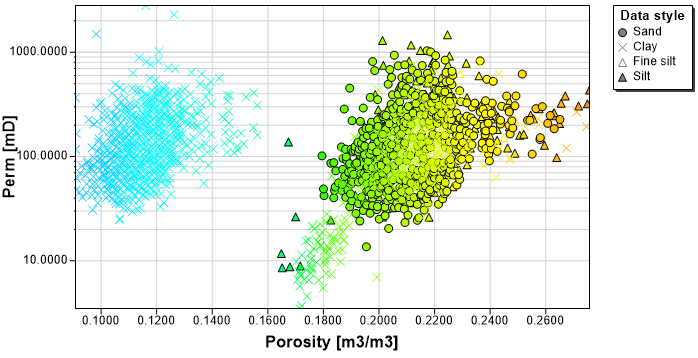
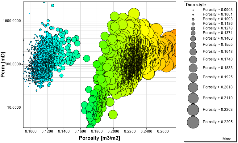
[The Blueback Investigator allows plotted points to be displayed using different shapes and shape sizes. For example, colored by dataset with different shapes based on facies.]
[The appearance shape can be changed using the context menu for the relevant. For continuous data, the number of shape data is divided between can be controlled from the legend context menu.]
[Appearance by dataset]{.underline}
[
 {width="6.197916666666667in" height="3.1770833333333335in"}]
[Appearance by discrete data or classification]{.underline}
[
 {width="6.197916666666667in" height="3.1770833333333335in"}]
[Color by continuous data]{.underline}
[
 {width="6.197916666666667in" height="3.7083333333333335in"}]{.underline}
[Contouring data]{.underline}
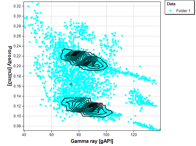
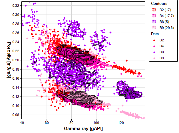
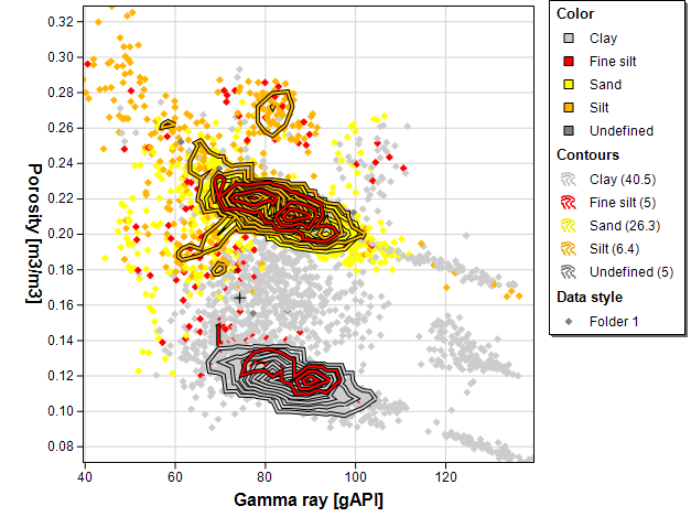
[Crossplots may contain a lot of points. If the density of these point clouds plots are high the points starts to be drawn on top of each other. The contour functionality draws contours on top of the point plot to identify areas where the points plot densely. Turn on contours by pressing the contour button in the toolbar.]
[The parenthesis displayed next to the Contour name in the legend contains the contour step for each contour. E.g. "]{.underline}[Sand (26.3)"]{.underline}[ means that you have 26.3 points in between each contour line. Control data will have effect on the contouring in the window.]
[Once displayed the contours can be exported to PDF's usable in Blueback Rock Physics.]
[Contours can be displayed for all data:]
[
 {width="6.197916666666667in" height="4.635416666666667in"}]
[Contours can be displayed per datasets:]
[
 {width="6.197916666666667in" height="4.635416666666667in"}]
[Contours can be displayed per discrete data type:]
[
 {width="6.197916666666667in" height="4.635416666666667in"}]
[Data highlighting]{.underline}
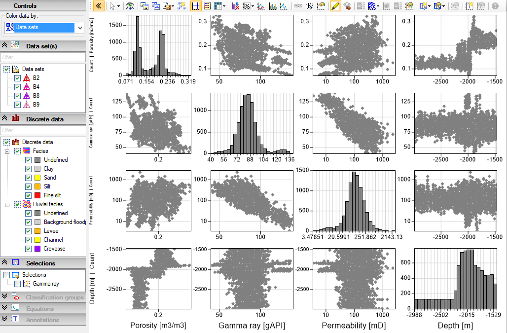
[Data highlighting mode allows the user to quickly and easily see how different data relates to the data within the investigation. ]
[The highlighted data is based on the selection in either the dataset, discrete data or classification group trees in the window control panel]{.underline}.
[Note: if selecting a child dataset of a folder like a well in a wells folder then the color by children setting is important. If the children of the folder are being colored by the folder then selecting to highlight a child will cause the entire folder dataset to be highlighted. To highlight just the child it is necessary to toggle the color by children option for the dataset.]
[Only the highlight data is used to determine best fit equations. This means that the dynamic equations will update when the highlight data is changed.]
[With no highlight data selected the window contains only grey data.]
[
 {width="5.354166666666667in" height="3.5208333333333335in"}]
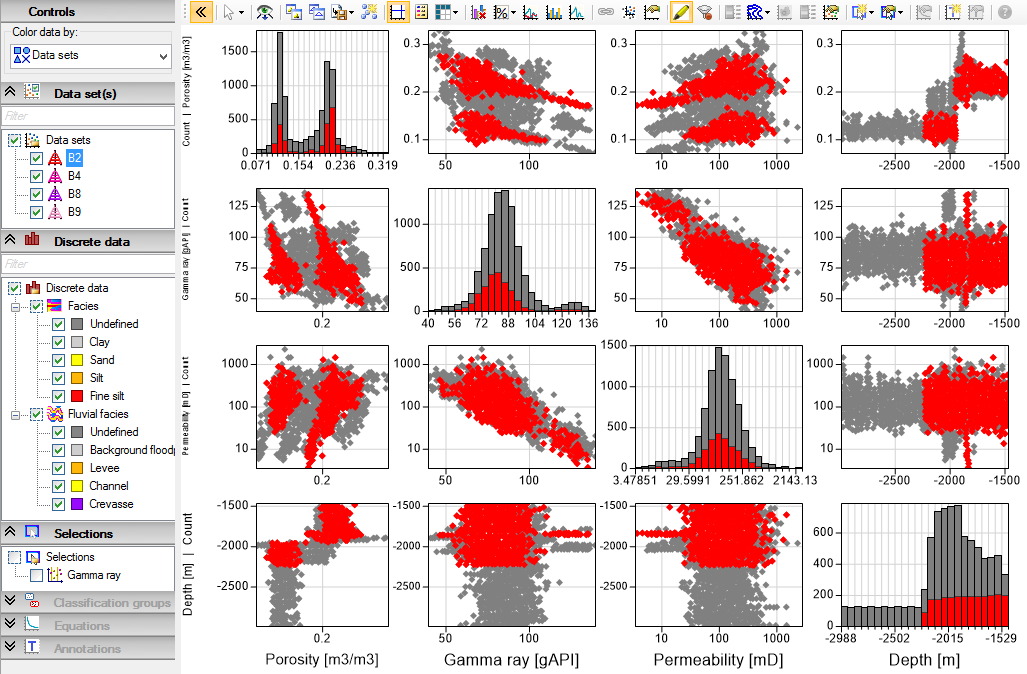
[By selecting the B2 well, the data from dataset B2 is colored by the chosen color by option. All other data remains grey.]
[
 {width="5.354166666666667in" height="3.5104166666666665in"}]
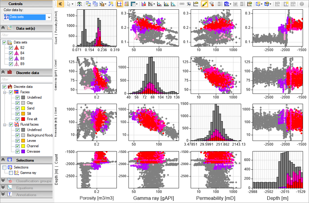
[By selecting the sand facies in the discrete data, the sand data is colored by the chosen color by option. All other data remains grey.]
[
 {width="5.364583333333333in" height="3.53125in"}]
[The data highlighting]{.underline} toolbar allows data highlighting mode to be toggled on/off. It also allows the unhighlighted data to be excluded from the plot if the user wishes.
[Selections]{.underline}
[Selections are user-specified areas inside Blueback Investigator windows that can function as filters or classifications.]
[Selections can be made using the following methods:]
- Blueback Investigator contains the following selection types:
[Note: Histograms are 1D data plots and as such can only support 1D selections]{.underline}
[Note: Scatterplots are 2D data plots and as such can support 1D, rectangle, polygon, freehand and ellipse selections]
[Note: 3D plots only support box and ellipsoid selections]
[Note: Selections are applied to the underlying data samples based on the linear/logarithmic settings of the dimension templates and not the how the dimension is currently displayed. This is important for 2D selections. The lines between 2D selection points are always drawn as straight lines. If the dimension is viewed in a different space to the original template then it is possible for the selected points to no longer match the extents of the selection in this space. ]
[
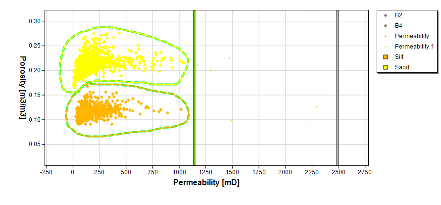 {width="6.197916666666667in" height="2.875in"}]
[An inverted horizontal 1D filter (in green) is used together with two freehand classifications to mark the areas as silt and sand.]{.underline}
[Filters]{.underline}
[Filters allow ranges of data to be selected within a plot. Blueback Investigator supports the following filter types:]
[1D horizontal axis filter]
[1D vertical axis filter]
[Rectangle filter]
[Freehand filter]
[Polygon filter]
[Ellipse filter]
[Box filter]
[Ellipsoid filter]
[The horizontal and vertical axis filters are 1D filters i.e. they filter the data in a single dimension only.]
[The rectangle, freehand, polygon and ellipse filters are 2D filters. ]
[The box and ellipsoid filters are 3D filters. ]
[When selected in the plot window (via the
 {width="0.25in" height="0.16666666666666666in"}drop down menu), filters are applied to all the data in the current Blueback investigation. In the example below, a rectangle filter has been applied to net/gross against permeability data in a scatterplot window. Points outside the rectangle are plotted brown to indicate they have been deselected by the filter whereas points inside the filter continue to be displayed in the default style (purple in this example)]
[Terminology]{.underline}
[The following terminology is used:]
[Filtered points]{.underline}[: Points reside outside of the filter. These are colored by the filter color.]
[Inverted filtered points:]{.underline}[ Points reside inside of the filter.]
[
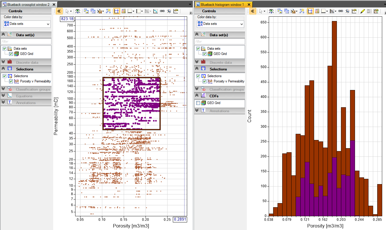 {width="6.197916666666667in" height="3.6875in"}]
[Multiple filters can be added to Blueback Investigator plot windows including filters of different types e.g. a crossplot may contain a horizontal cut-off filter and a freehand filter. Other selections can also be added.]
[Filters will only be visible in the data template space in which they have been created. In the example above a rectangular filter has been created in a net/gross vs permeability plot and as such the filter lines will only be displayed in a net/gross vs permeability plot. However, the effects of the filter can be seen in any data template space for the current Blueback investigation. For example, the histogram above is displaying porosity data but the net/gross vs permeability filter is available and has been selected. The filter itself is not shown but the effects of it are visible in the histogram with the porosity data corresponding to the points within the rectangle filter on the scatterplot displayed in purple and the remainder of the data displayed in brown.]
[Petrel filters vs Blueback filters]{.underline}
[The main reason for implementing Blueback filters is the lack of filter support for some of the key data types we support in Blueback Investigator.]
[Most of the above filter types are available in two flavors: ]
[Blueback filters are local to the current Blueback investigation and are not available outside of the Blueback Investigator]
[Petrel filters are stored in the Petrel project so can be used in multiple places, including in Blueback Investigator plots. ]
- [However, in order to display a Petrel filter in the Blueback Investigator a linked Blueback filter must be created. This can be done in one of two ways, depending on how the Petrel filter is created:]
[Blueback filters can be created from existing Petrel filters via the ]{.underline}[Save as Blueback filter]{.underline}[ option on the Petrel filter context menu. The user will be prompted to select the Blueback investigation in which to create the Blueback filter; any existing Blueback investigation containing a compatible data template space can be selected]
[Petrel filters can be digitized direct from a Blueback Investigator plot window (in the same manner as in the Petrel histogram and function windows) in which case a linked Blueback filter will automatically be created.]
[As well as being able to create Blueback filters from Petrel filters one is also able to create Petrel filters from existing Blueback filters by right-clicking on a Blueback filter (e.g. the Net/Gross v Permeability filter shown in the histogram dropdown above) and selecting ]{.underline}[Save as Petrel filter]{.underline}[ from the context menu.]
[The link between Blueback and Petrel filters applies to the extents of the filter but not the color. For example, changing the maximum limit of a Petrel filter will change the maximum extent of the linked Blueback filter too but changing the color of one will not change the color of the other.]
[N.B.]{.underline}[ Due to a limitation in Ocean there is no option to create rectangular Petrel filters from within Blueback plots. Instead all 2D Petrel filters created from Blueback plots or via the ]{.underline}[Save as Petrel filter]{.underline}[ option are freehand filters. This means that while rectangular Blueback filters can be saved as Petrel filters the result will be rectangular initially but the Petrel filter is not constrained to remain rectangular.]
[Classifications]{.underline}
[Classifications allow ranges of data to be selected within a plot to assign discrete codes to a selection area. The classified points can be used in other parts of Petrel, for instance with the Upscale well logs process if you would like to make new 3D property based on your classification input.]
[The Blueback Investigator supports the following classification types:]
[1D horizontal axis classification]
[1D vertical axis classification]
[Rectangle classification]
[Freehand classification]
[Polygon classification]
[Once a classification is defined, the points inside the selections can be colored by the classification codes. By default this is turned off.]
[
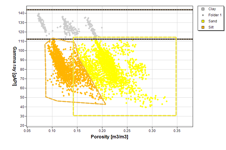 {width="6.197916666666667in" height="4.125in"}]
[Simple classification workflow using a discrete facies template to highlight possible classification areas that relate to a discrete parameter.]{.underline}
[Discrete templates and Classification groups]{.underline}
[Discrete templates are used in the classification workflow. In the image above a simple facies classification is performed using a Classification group]{.underline}.
[The Classification group is a special user defined discrete template that can be based on a Petrel template. To assign values to a classification it should be tied to a classification group. Classification groups are defined in the investigation or from right clicking on a ]{.underline}[unclassifed]{.underline}[ classification selection (Black color).]
[The Classification group contains 2 built-in discrete codes, Filtered and Unclassified.]
[
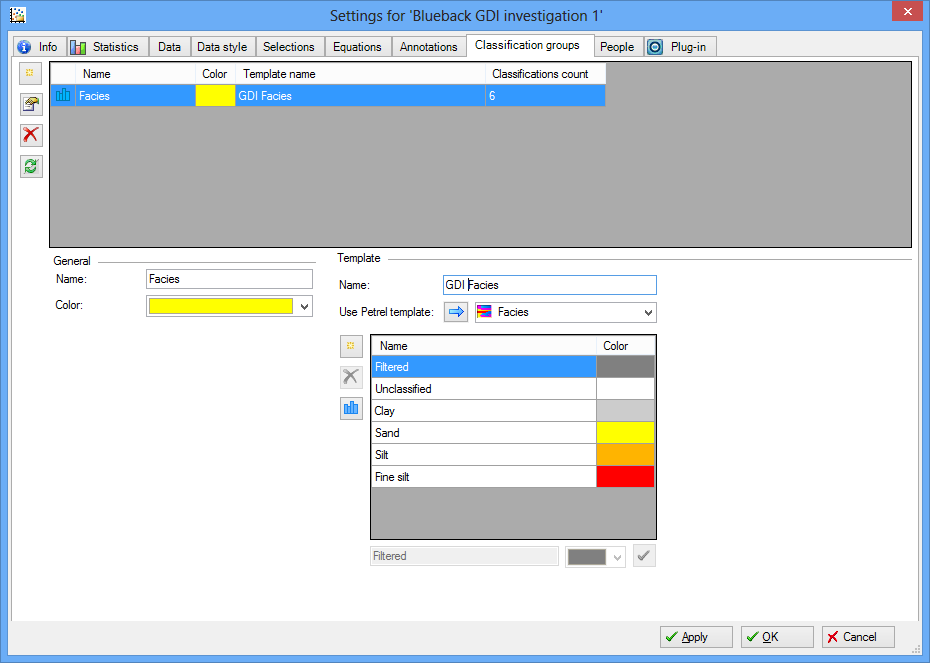 {width="6.197916666666667in" height="4.416666666666667in"}]
[A new Classification group based on the Petrel Facies template is created inside the investigation.]{.underline}
[Selection priority]{.underline}
[In Blueback Investigator two selection types exist, filters and classifications. In the investigation the priority the selections have can be set. Filters always take priority over classified regions, even if the filter is added after the classified region or the user changes the priorities in the investigation. This is by design. ]
[Classified regions allow the user to ]{.underline}[tag]{.underline}[ points as belonging to a certain discrete classification whereas filters allow users to exclude points as being of no real interest. If the user excludes a point with a filter it is not included in the classification.]
[Example]{.underline}
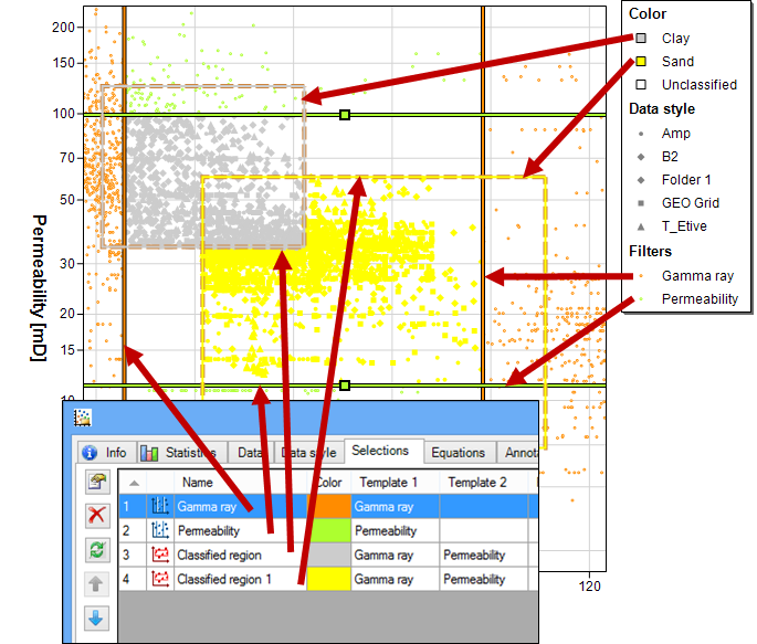
[An investigation has four selections: Two 1D filters and two 2D classified areas:]
[
 {width="6.197916666666667in" height="5.270833333333333in"}]
[The selection priority is set in the Selections settings dialog: ]
[In the image above all the points outside of the filters will be are inactive.]
[Filters take priority over classifications. Permeability and Gamma ray filters defines the active points.]
[Two classifications overlap, the priority in the investigation is reflected in the plot and the legend]
[1D Horizontal axis selection method]{.underline}
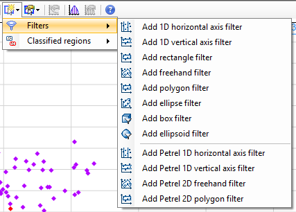
[A 1D Horizontal axis selection can be created by first selecting the ]{.underline}[Add selection]{.underline}[ option, followed by selection of the appropriate selection type submenu and then ]{.underline}[Add 1D horizontal axis ]{.underline}[option:]
[
 {width="4.447916666666667in" height="3.1875in"}]
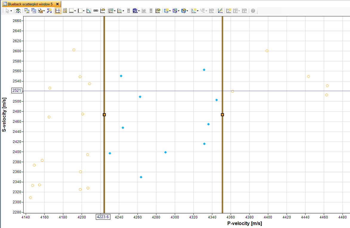
[This selection method is drawn in a plot window as follows: ]
[Click (and hold) on a point to start drawing the horizontal selection. ]
[Move the mouse to the intended edge of the selection. ]
[Release the mouse to confirm the edge of the selection.]
[
 {width="6.197916666666667in" height="4.052083333333333in"}]
[The edges of the selection can be expanded or contracted after the selection has been drawn by first mousing over the central square icon of the selection edges, followed by a drag and drop action to the new edge position. ]
[The selection as a whole can be dragged to a new position by first mousing over a portion of one of the selection edges (away from the central square icon), followed by a drag and drop action to the new selection position.]
[1D Vertical axis selection method]{.underline}
[A 1D Vertical axis selection can be created by first selecting the ]{.underline}[Add selection]{.underline}[ option, followed by selection of the appropriate selection type submenu and then ]{.underline}[Add 1D vertical axis ]{.underline}[option:]
[
{width="4.447916666666667in" height="3.1875in"}][This selection method is drawn in a plot window as follows: ]
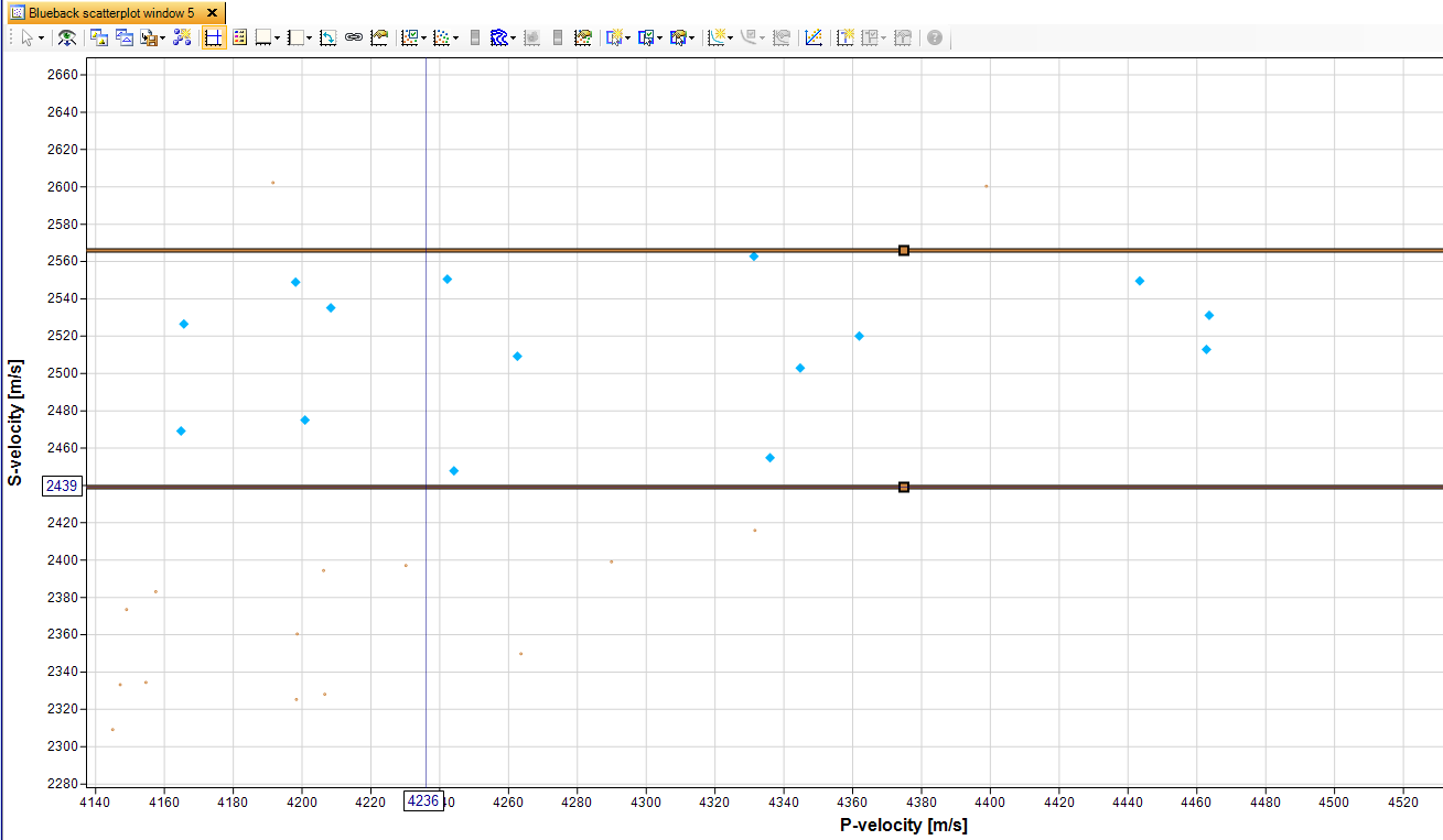
[Click (and hold) on a point to start drawing the vertical selection. ]
[Move the mouse to the intended edge of the selection. ]
[Release the mouse to confirm the edge of the selection.]
[
 {width="6.197916666666667in" height="3.6041666666666665in"}]
[The edges of the selection can be expanded or contracted after the selection has been drawn by first mousing over the central square icon of the selection edges, followed by a drag and drop action to the new edge position. ]
[The selection as a whole can be dragged to a new position by first mousing over a portion of one of the selection edges (away from the central square icon), followed by a drag and drop action to the new selection position.]
[Rectangle selection method]{.underline}
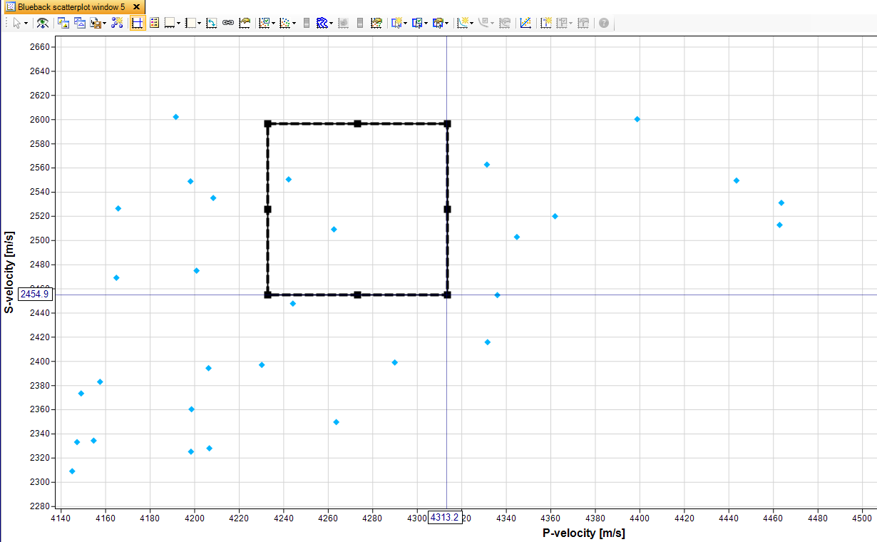
[A rectangular selection can be created by first selecting the ]{.underline}[Add selection]{.underline}[ option, followed by selection of the appropriate selection type submenu and then ]{.underline}[Add rectangle ]{.underline}[option:]
[
{width="4.447916666666667in" height="3.1875in"}][This selection method is drawn in the plot window as follows: ]
[Click (and hold) the mouse at one of the corners of the intended rectangular selection.]
[Drag the mouse to the opposite corner of the intended rectangular selection.]
[Release the mouse to confirm the rectangular shape created.]
[
 {width="6.197916666666667in" height="3.8229166666666665in"}]
[The corners and edges of the rectangular selection can be expanded or contracted to define a new area. This is done by first mousing over one of the relevant square icons at the edges and corners and then performing a click and drag action to a new position.]
[The selection as a whole can be dragged to a new position. This is done by first mousing over one of the edges away from any square icon and then performing a click and drag action to a new position.]
[Polygon selection method]{.underline}
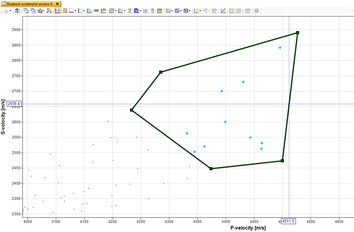
[A polygon selection can be created by first selecting the ]{.underline}[AAdd selection]{.underline}[ option, followed by selection of the appropriate selection type submenu and then ]{.underline}[Add polygon ]{.underline}[option:]
[
{width="4.447916666666667in" height="3.1875in"}][This selection method can be drawn in a plot window as follows:]
[Click and release once and the intended start point of the polygon selection.]
[Move the mouse cursor to the next intended point of the polygon selection. A guideline is drawn to show where the next polygon selection edge would be placed.]
[Click and release the mouse to add another polygon point.]
[Continue to add points until the intended shape is created. ]
[Double click to confirm the last point of the polygon. A final edge is created from the final point to the starting point.]
[Only polygons with three or more points are permitted. Those with fewer points are removed.]
[Pressing the ]{.underline}[Escape]{.underline}[ keyboard key at any time before step 6 will cause the most recently drawn point to act as the final point of the selection. (Or remove the polygon entirely if less than three points have been created.) ]
[Following the drawing of the polygon selection, a dialog appears prompting you to choose whether to remove unnecessary control points. Choosing this option means that only the minimum number of points that define the selection shape created will be kept. This simplification can also be performed at a later point (by right clicking on the completed polygon selection and choosing the ]{.underline}[Simplify]{.underline}[ option from the context menu for that selection).]
[
 {width="6.197916666666667in" height="4.0625in"}]
[A completed polygon selection can be modified in a number of ways: ]
[Individual control points can be dragged to new positions. This is achieved by mousing over one of the selection control points, followed by a click and drag action to a new position.]
[The selection as a whole can be dragged to a new position. This is achieved by mousing over part of the selection away from any control points, followed by a click and drag action to a new position. ]
[Individual control points can be deleted. This is achieved by right clicking on the control point, followed by selecting the ]{.underline}[Delete Selection Point]{.underline}[ option. (Alternatively, you can mouse over a point for deletion and press the ]{.underline}[Delete]{.underline}[ key on the keyboard.) If this action would result in a polygon with fewer than 3 points, a dialog appears and prompts you whether to remove the polygon entirely.]
[Individual control points can be added. This is achieved by right clicking on an edge of the selection that does not contain a point, followed by selecting the ]{.underline}[Add Selection Point]{.underline}[ option.]
[Freehand selection method]{.underline}
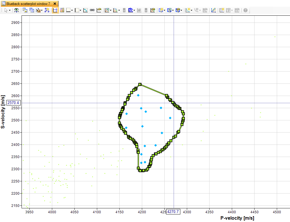
[A rectangular selection can be created by first selecting the ]{.underline}[Add selection]{.underline}[ option, followed by selection of the appropriate selection type submenu and then ]{.underline}[Add freehand ]{.underline}[option:]
[
{width="4.447916666666667in" height="3.1875in"}][This selection method can be drawn in a plot window as follows: ]
[Click (and hold) the mouse at the start position of the selection.]
[Drag the mouse in the shape you wish to define. A freehand selection will follow the path of the mouse precisely. ]
[Release the mouse once the shape is complete. A final edge will be drawn automatically, linking the start and end positions of the selection.]
[Following the drawing of the freehand selection, a dialog appears prompting you to choose whether to remove unnecessary control points. Choosing this option means that only the minimum number of points that define the path of the mouse during the drawing phase will remain. This simplification can also be performed at a later point (by right clicking on the completed freehand selection and choosing the ]{.underline}[Simplify]{.underline}[ option from the context menu for that selection).]
[
 {width="6.197916666666667in" height="4.739583333333333in"}]
[A completed freehand selection can be modified in a number of ways: ]
[Individual control points can be dragged to new positions. This is achieved by mousing over one of the selection control points, followed by a click and drag action to a new position.]
[The selection as a whole can be dragged to a new position. This is achieved by mousing over part of the selection away from any control points, followed by a click and drag action to a new position. ]
[Individual control points can be deleted. This is achieved by right clicking on the control point, followed by selecting the ]{.underline}[Delete Selection Point]{.underline}[ option. (Alternatively, you can mouse over a point for deletion and press the ]{.underline}[Delete]{.underline}[ key on the keyboard.)]
[Individual control points can be added. This is achieved by right clicking on an edge of the selection that does not contain a point, followed by selecting the ]{.underline}[Add Selection Point]{.underline}[ option.]
[Ellipse selection method]{.underline}
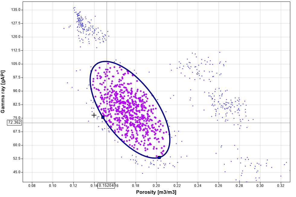
[A 2D ellipse selection can be created by first selecting the ]{.underline}[Add selection]{.underline}[ option, followed by selection of the appropriate selection type submenu and then ]{.underline}[Add 2D ellipse]{.underline}[ option:]
[
{width="4.447916666666667in" height="3.1875in"}][This selection method is drawn in the plot window as follows: ]
[Click (and hold) the mouse at the centre of the intended ellipse selection.]
[Drag the mouse to define the orientation and magnitude of the primary axis of the ellipse selection.]
[Release the mouse to confirm the ellipse shape created.]
[
 {width="6.197916666666667in" height="4.125in"}]
[The magnitude and orientation of the ellipse can be modified to define a new area. This is done by first mousing over one of the relevant square icons on the edge and then performing a click and drag action to a new position.]
[The selection as a whole can be dragged to a new position. This is done by first mousing over the edge away from any square icon and then performing a click and drag action to a new position.]
[Box selection method]{.underline}
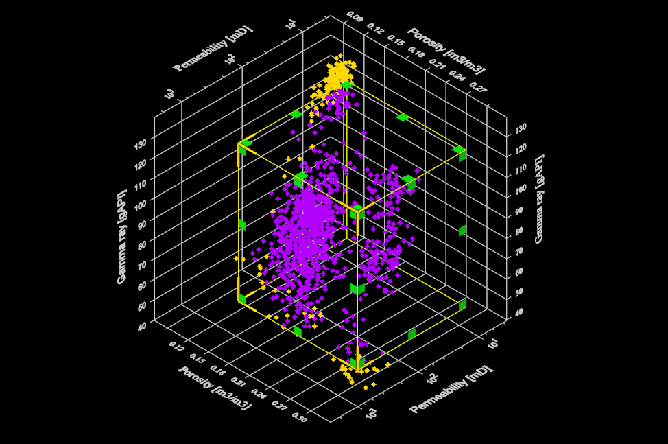
[A 3D box selection can be created by first selecting the ]{.underline}[Add selection]{.underline}[ option, followed by selection of the appropriate selection type submenu and then ]{.underline}[Add box]{.underline}[ option:]
[
{width="4.447916666666667in" height="3.1875in"}][A box selection will be created in the 3D plot. ]
[
 {width="6.197916666666667in" height="4.114583333333333in"}]
[When the 3D plot is in pick mode the green tabs will be visible to allow manipulation. ]
[The corners and edges of the box selection can be expanded or contracted to define a new area. This is done by first mousing over one of the relevant green tabs at the edges and corners and then performing a click and drag action to a new position.]
[The selection as a whole can be dragged to a new position. This is done by performing a click inside the box and dragging to a new position. ]{.underline}[Note: It is sometime difficult to move the box if a lot of data is displayed.]{.underline}
[Ellipsoid selection method]{.underline}
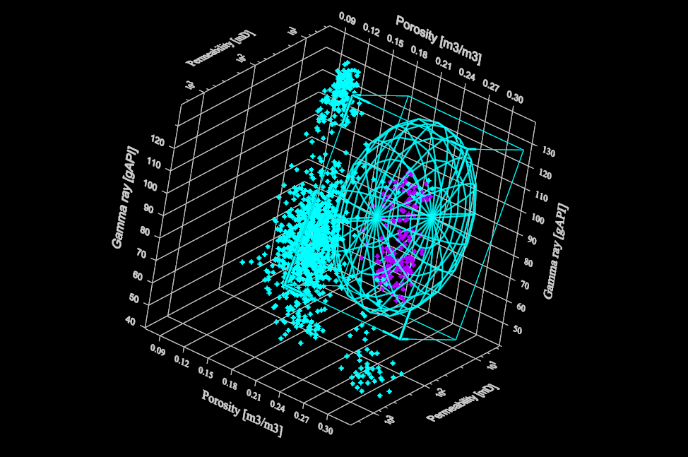
[A 3D ellipsoid selection can be created by first selecting the ]{.underline}[Add selection]{.underline}[ option, followed by selection of the appropriate selection type submenu and then ]{.underline}[Add ellipsoid]{.underline}[ option:]
[
{width="4.447916666666667in" height="3.1875in"}][An ellipsoid selection will be created in the 3D plot.]
[
 {width="6.197916666666667in" height="4.114583333333333in"}]
[When the 3D plot is in pick mode the green tabs and rotate arrows will be visible to allow manipulation. ]
[The corners and edges of the box can be expanded or contracted to define a new area. The ellipsoid will fill this box. This is done by first mousing over one of the relevant green tabs at the edges and corners and then performing a click and drag action to a new position.]
[The selection as a whole can be dragged to a new position. This is done by performing a click inside the box and dragging to a new position. ]{.underline}[Note: It is sometime difficult to move the box if a lot of data is displayed.]{.underline}
[The selection can be rotated. This is done by performing a click on one of the green rotation arrows and dragging to a new position. ]{.underline}[Note: It is sometime difficult to rotate the box if a lot of data is displayed.]{.underline}
[Timespan classifications]{.underline}
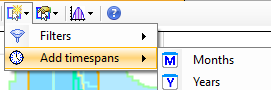
[Investigations with time-series datasets support timespan classifications. These can be added from the selections toolbar button.]
[
 {width="2.8229166666666665in" height="0.9375in"}]
[The options allow the user to quickly create either a classification by month or by year based on the date dimension. These classifications can be used on all windows allowing the data to be quickly split and analysed by smaller timespans if required.]
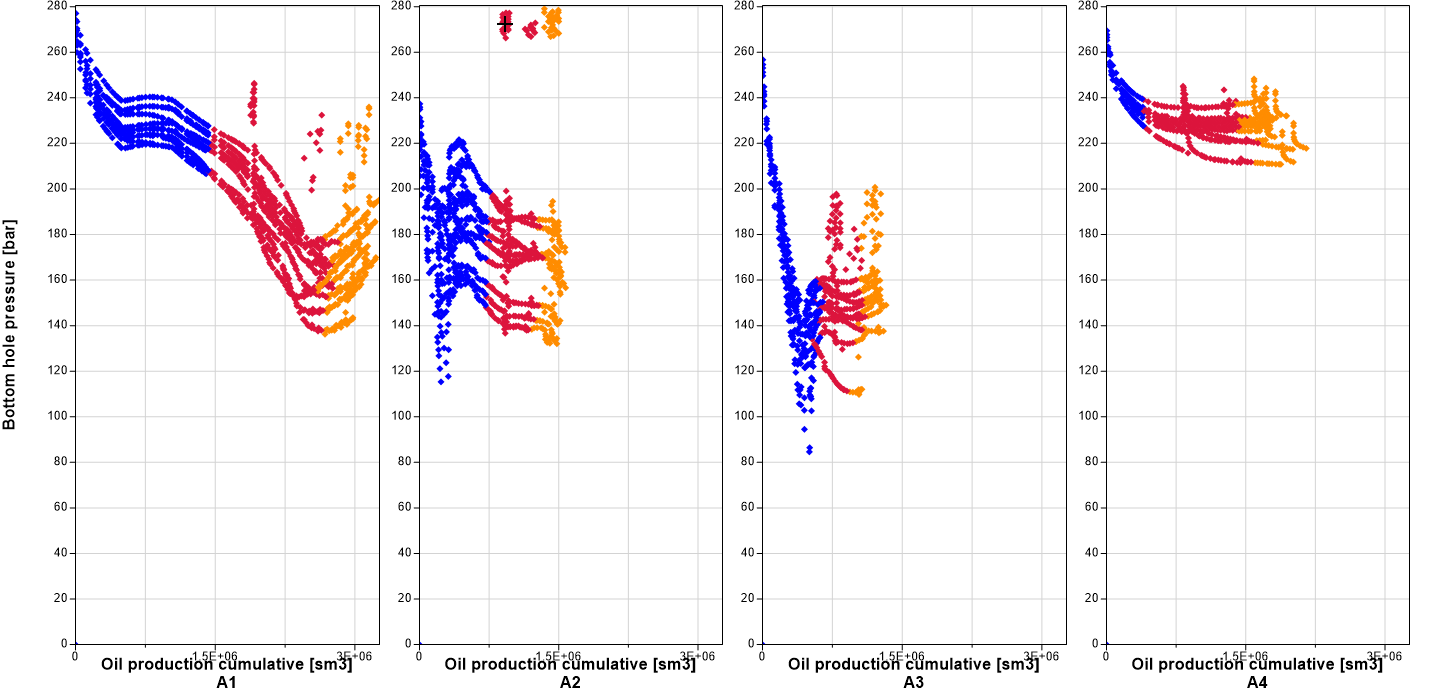
[For example, this plot shows cumulative oil production v bottom hole pressure for 4 wells colored by the different year timespans.]
[
 {width="6.197916666666667in" height="3.0104166666666665in"}]
[Equations]{.underline}
[An equation is a mathematical concept describing the relationship between two data quantities, x and y. In other words, it indicates how y may be calculated based on known x data. In the Blueback Investigator it is this relationship that is stored as opposed to a set of (x,y) points conforming to the relationship between the two quantities, which is how Petrel functions are stored. This makes Blueback Investigator equations more powerful than Petrel functions.]
[NB]{.underline}[ The Blueback equation can only be saved in Blueback investigations containing compatible data templates.]
[An equation is specified as either y = f(x) or x = f(y). The equation stores the X and Y templates against which it is defined. This information is used when calculating the equation to ensure the correct output data is determined using the input data irrespective of the plot axis orientation. ]
[An equation can be drawn in any plot space in which it is valid.]
[The list of supported equation types can be found here]{.underline}.
[A description of how Petrel functions and Blueback equations are related can be found here]{.underline}.
[Equation types]{.underline}
[A variety of equation lines can be added to all Blueback Investigator plots except histograms and parallel coordinates plot:]
[simple regression analysis (for more information see Simple regression analysis]{.underline})
[user-defined equations (for more information see User defined equations]{.underline})
[user expression equations (for more information see User expression equations]{.underline})
[Bayesian classification (for more information see Bayesian classification]{.underline})
[Multi-linear regression (for more information see Multi-linear regression]{.underline})
[K-means classification (for more information see Kmeans classification]{.underline})
[python script equations (for more information see Prizm Investigator]{.underline})
[Simple regression analysis]{.underline}
[The following simple regressions (best fits) can be calculated:]
[linear best fit line]
[Ordinary least squares regression]
[Total least squares regression]
[Reduced major axis regression]
[Walden robust fit regression]
[logarithmic best fit line]
[power law best fit line]
[exponential best fit line]
[polynomial best fit line]
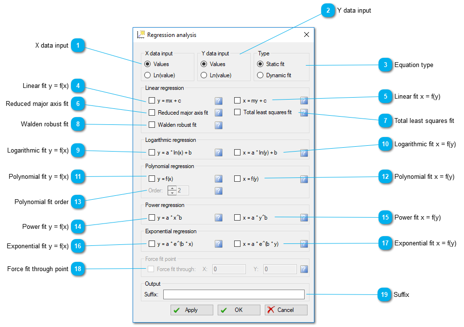
[The fits to be calculated are controlled from the Simple regression analysis dialog]{.underline}.
[All best-fit lines are fitted to the currently selected data. ]
[The best fit equations can be either static or dynamic (for more information see Static v dynamic equations]{.underline}).
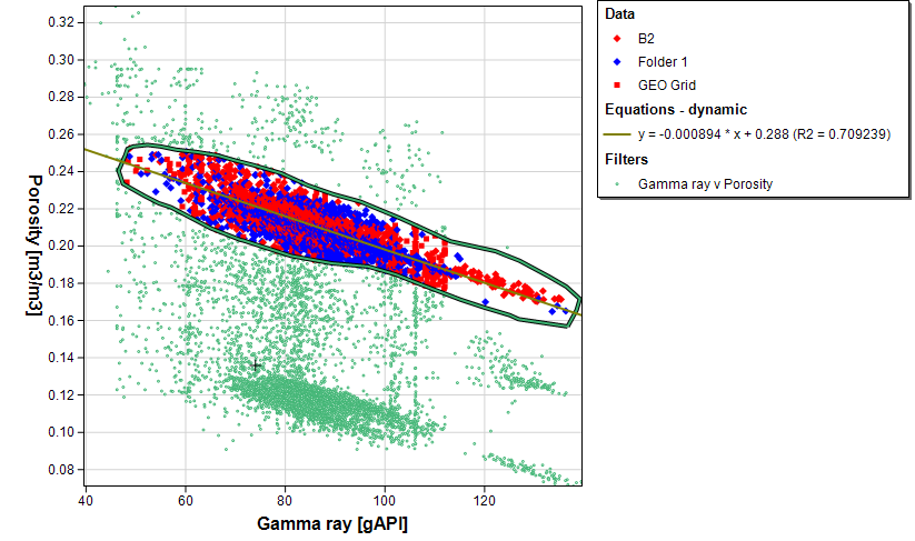
[The gamma ray vs porosity scatterplot below shows a freehand filter being used to select a group of data points. The blue linear best fit line has then been fitted to only the selected points rather than the full dataset. This equation is dynamic so if the filter is changed then the best fit will be recalculated.]
[
 {width="6.197916666666667in" height="3.6666666666666665in"}]
[Simple regression analysis dialog]{.underline}
[
 {width="6.197916666666667in" height="4.364583333333333in"}]
[
 {width="0.4166666666666667in" height="0.4166666666666667in"}]{.underline}[X data input]{.underline}
[
 {width="1.2083333333333333in" height="0.7604166666666666in"}]
[Use either the raw values or the natural logarithm of the values for X.]
[Note: The calculated equation can be displayed in either natural log or log base 10 as required]
[
 {width="0.4166666666666667in" height="0.4166666666666667in"}]{.underline}[Y data input]{.underline}
[
 {width="1.1770833333333333in" height="0.7708333333333334in"}]
[Use either the raw values or the natural logarithm of the values for Y.]
[Note: The calculated equation can be displayed in either natural log or log base 10 as required]
[
 {width="0.4166666666666667in" height="0.4166666666666667in"}]{.underline}[Equation type]{.underline}
[
 {width="1.2291666666666667in" height="0.7916666666666666in"}]
[Create either static of dynamic best fits (see Static v dynamic equations]{.underline})
[
 {width="0.4166666666666667in" height="0.4166666666666667in"}]{.underline}[Linear fit y = f(x)]{.underline}
[
 {width="0.875in" height="0.28125in"}]
[Create an ordinary least squares linear fit from the X values]
[
 {width="0.4166666666666667in" height="0.4166666666666667in"}]{.underline}[Linear fit x = f(y)]{.underline}
[
 {width="0.875in" height="0.28125in"}]
[Create an ordinary least squares linear fit from the Y values]
[
 {width="0.4166666666666667in" height="0.4166666666666667in"}]{.underline}[Reduced major axis fit]{.underline}
[
 {width="1.4166666666666667in" height="0.28125in"}]
[Create a reduced major axis fit. ]
[This is a linear regression that minimizes the error in both X and Y.]
[
 {width="0.4166666666666667in" height="0.4166666666666667in"}]{.underline}[Total least squares fit]{.underline}
[
 {width="1.4375in" height="0.2916666666666667in"}]
[Create a total least squares fit.]
[This is a linear regression that minimizes the error in both X and Y when the data is normalized.]
[
 {width="0.4166666666666667in" height="0.4166666666666667in"}]{.underline}[Walden robust fit]{.underline}
[
 {width="1.2083333333333333in" height="0.28125in"}]
[Create a Walden robust fit.]
[Walden' (1991) robust fitting minimizes the effects of outliers by first creating a fit between the medians of the left and right-hand sides of the displayed data, and then uses weighted least-squares regression to fit the points, each weighted by their distance to the initial fit line. It uses the Andrews (1972, 1974) method to reduce or completely eliminate the influence of large residuals]
[
 {width="0.4166666666666667in" height="0.4166666666666667in"}]{.underline}[Logarithmic fit y = f(x)]{.underline}
[
 {width="1.1041666666666667in" height="0.28125in"}]
[Create a logarithmic fit from the X values]
[
 {width="0.4166666666666667in" height="0.4166666666666667in"}]{.underline}[Logarithmic fit x = f(y)]{.underline}
[
 {width="1.1041666666666667in" height="0.28125in"}]
[Create a logarithmic fit from the Y values]
[
 {width="0.4166666666666667in" height="0.4166666666666667in"}]{.underline}[Polynomial fit y = f(x)]{.underline}
[
 {width="0.6979166666666666in" height="0.28125in"}]
[Create a polynomial fit from the X values using the order specified]
[
 {width="0.4166666666666667in" height="0.4166666666666667in"}]{.underline}[Polynomial fit x = f(y)]{.underline}
[
 {width="0.6979166666666666in" height="0.28125in"}]
[Create a polynomial fit from the Y values using the order specified]
[
 {width="0.4166666666666667in" height="0.4166666666666667in"}]{.underline}[Polynomial fit order]{.underline}
[
 {width="1.0in" height="0.28125in"}]
[Specifies the order of the polynomial fit to be created]
[
 {width="0.4166666666666667in" height="0.4166666666666667in"}]{.underline}[Power fit y = f(x)]{.underline}
[
 {width="0.8958333333333334in" height="0.28125in"}]
[Create a power fit from the X values]
[
 {width="0.4166666666666667in" height="0.4166666666666667in"}]{.underline}[Power fit x = f(y)]{.underline}
[
 {width="0.8958333333333334in" height="0.28125in"}]
[Create a power fit from the Y values]
[
 {width="0.4166666666666667in" height="0.4166666666666667in"}]{.underline}[Exponential fit y = f(x)]{.underline}
[
 {width="1.125in" height="0.28125in"}]
[Create an exponential fit from the X values]
[
 {width="0.4166666666666667in" height="0.4166666666666667in"}]{.underline}[Exponential fit x = f(y)]{.underline}
[
 {width="1.125in" height="0.28125in"}]
[Create an exponential fit from the Y values]
[
 {width="0.4166666666666667in" height="0.4166666666666667in"}]{.underline}[Force fit through point]{.underline}
[
 {width="3.28125in" height="0.28125in"}]
[Optionally, force certain regressions through a given point (for example the origin 0, 0)]
[
 {width="0.4166666666666667in" height="0.4166666666666667in"}]{.underline}[Suffix]{.underline}
[
 {width="3.09375in" height="0.2708333333333333in"}]
[Defines the suffix to be added to the created equation names]
[User defined equations]{.underline}
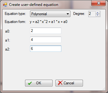
[User-defined equations allow the user to specify the equation type and the various coefficients to define the equation pre-defined equation forms. ]
[User-defined equations are always static equations.]
[The following equation types are supported:]
[linear]
[logarithmic]
[power law]
[exponential]
[polynomial]
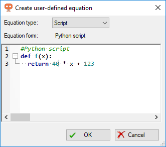
[python]
[This allows the user to compare their data against any relationship between the plotted quantities. For example, a published relationship could be added as a user-defined equation.]
[
 {width="3.59375in" height="3.125in"}]
[User-defined equations are editable and can be moved and adjusted. Static and dynamic equations can be made editable by converting them to a user defined equation.]
[User defined python equation]{.underline}
[Blueback Investigator has an option to read simple python scripts and use them as an user defined equation.]
[
 {width="3.4479166666666665in" height="3.0520833333333335in"}]
[More information about the functionality:]
- [The function should always be a function of x.]
- [The inputs and outputs of the function must be in system invariant (SI) units rather than display units. This is necessary to allow the equation to be displayed no matter what units are being used in the plot.]
[Currently the flavor of python that is used is IronPython.]
[For more information on the syntax take a look here: http://en.wikibooks.org/wiki/Python_Programming/Basic_Math]
[User expression equations]{.underline}
[User-defined expression equations allow the user to specify any equation they require. The equation is written in a calculator style eg $A + ($B * $C).]
[User-defined expression equations are always static equations. ]
[As these equations can have more than 1 input dimension, they will not be rendered on plots. The result of the equation can be included as a new dimension in the investigation. ]
[These equations can also be used in the Equation transformer tool]{.underline} or [weighting histograms]{.underline} or as [additional dimensions]
[The equation can be given a name and an template must be selected. ]
[Note: The equation should return results in the SI unit of the selected output template.]{.underline}
[Note: Any constants used in the equation should be specified in SI units.]{.underline}
[
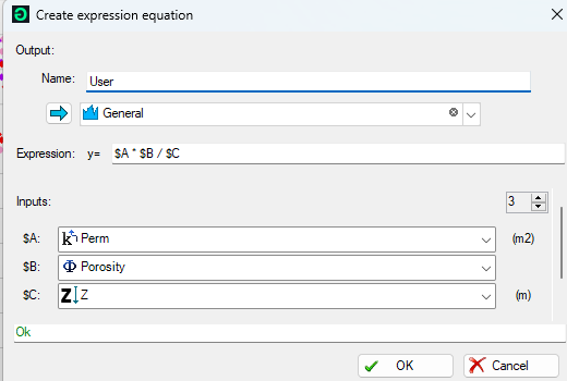 {width="5.416666666666667in" height="3.6458333333333335in"}]
[Bayesian classification]{.underline}
[Bayesian classification allows the statistical information representing different known classifications to be used to classify unknown data.]
[This equation performs classification and outputs discrete properties. This equation cannot be rendered on the plots.]
[A Bayesian classification can only be created from discrete data. The option will only be enabled when the data is displayed as discrete data.]
[A Bayesian classification equation parameters can be defined during creation using this dialog]{.underline}.
[For example, a Bayesian classification performed on well log data can be used to classify seismic inversion results.]
[Define Bayesian classification based on well logs]
[
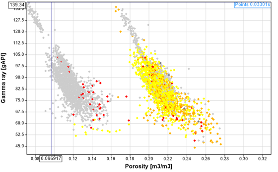 {width="5.833333333333333in" height="3.625in"}]
[Create a new discrete volume from the Bayesian classification]
[
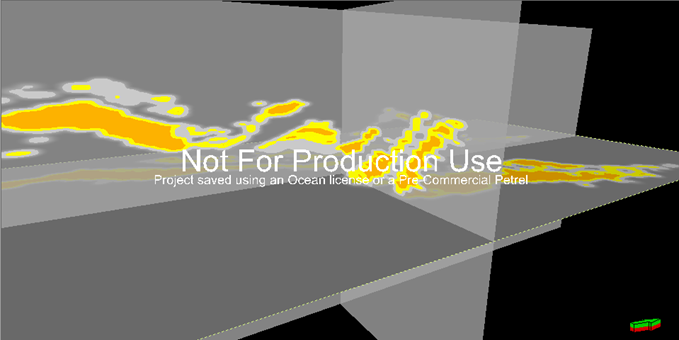 {width="6.197916666666667in" height="3.09375in"}]
[Create Bayesian classification dialog]{.underline}
[
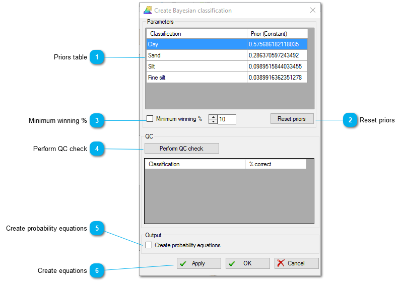 {width="6.197916666666667in" height="4.34375in"}]
[
{width="0.4166666666666667in" height="0.4166666666666667in"}]{.underline}[Priors table]{.underline}[
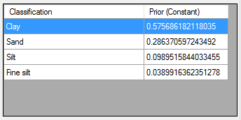 {width="3.5833333333333335in" height="1.7916666666666667in"}]
[This table allows the priors associated with each discrete classification. The default priors are calculated based on the relative proportions of the input data.]
[
{width="0.4166666666666667in" height="0.4166666666666667in"}]{.underline}[Reset priors]{.underline}[
 {width="1.0208333333333333in" height="0.34375in"}]
[This resets the priors to the default values.]
[
{width="0.4166666666666667in" height="0.4166666666666667in"}]{.underline}[Minimum winning %]{.underline}[
 {width="2.0520833333333335in" height="0.3333333333333333in"}]
[Allows a minimum winning percentage to be defined.]
[If checked then the probability of the winning Bayesian classification must be greater than the specified value to be used. If the probability is less than this value then the sample will the ]{.underline}[undefined]{.underline}[.]
[
{width="0.4166666666666667in" height="0.4166666666666667in"}]{.underline}[Perform QC check]{.underline}[
 {width="3.625in" height="1.8229166666666667in"}]
[Performs a QC check on the Bayesian classification equation. ]
[The data samples from which the statistics used in the equation were determined are classified using the Bayesian classification equation and compared to the actual input classification. The table shows the percentage of correct classifications for each discrete classification.]
[
{width="0.4166666666666667in" height="0.4166666666666667in"}]{.underline}[Create probability equations]{.underline}[
 {width="1.78125in" height="0.28125in"}]
[Creates probability equations for each discrete classification.]
[
{width="0.4166666666666667in" height="0.4166666666666667in"}]{.underline}[Create equations]{.underline}[
 {width="2.03125in" height="0.34375in"}]
[Creates the Bayesian classification equation and optional probability equations if selected.]
[Multi-linear regression]{.underline}
[Allows a new linear equation to be created that relates multiple input dimensions. This equation cannot be rendered on the plots.]
[The equation can be used to predict properties using the new calculated dimensions or equation transformer tool]
[The user can select which dimensions to include as input and output dimensions.]
[
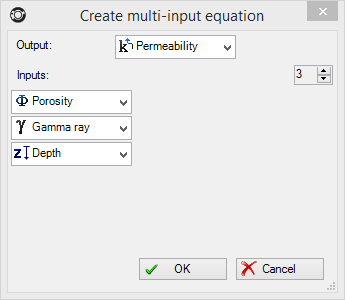 {width="3.59375in" height="3.125in"}]
[Kmeans classification]{.underline}
[The KMeans clustering algorithm can be used to identify clusters of points within the displayed data. More information about the KMeans clustering algorithm can be found here]{.underline}.
[The user defines the number of clusters to be identified and the algorithm divides the data into the required number of clusters. The definition of these clusters is stored as a classified equation within the investigation. A new classification group is automatically created defining the classifications for the required number of clusters. ]
[The algorithm will use all the displayed continuous dimensions to determine the clusters. An N-dimensional Kmeans classification can therefore be created from the matrix window, a 2D K-means classification will be created from the crossplot window.]
[Prior to version 5.5, Kmeans classifications were stored as classified regions which could be edited by the user as necessary to refine the classifications.]
[Note: The algorithm gives the best results on well separated data. If the user asks for 10 clusters then the algorithm will identify 10 clusters even if there does not appear to be relationships within the clusters to the human eye]{.underline}
[
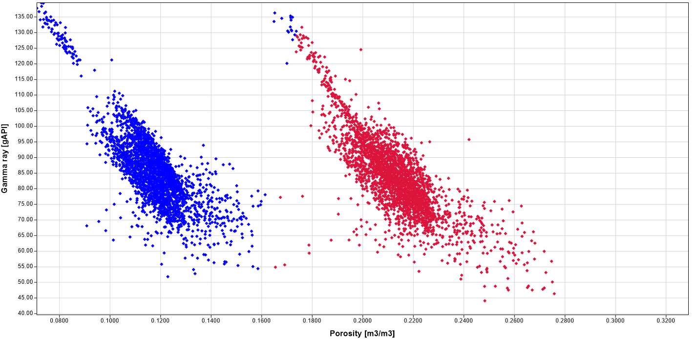 {width="6.197916666666667in" height="3.0in"}]
[Static v dynamic equations]{.underline}
[What is a static equation?]{.underline}
[A static equation does not change when the displayed data changes and is not impacted by subsequent filtering.]
[If a static best fit equation is created then the equation is based on the snapshot of the data displayed at the time of creation.]
[A static best fit equation can be changed into a dynamic equation. If the static equation is displayed in more than one window then it will be toggled off in all but one of these windows.]
[What is a dynamic equation?]{.underline}
[A dynamic equation changes with the displayed data is changed and is impacted by subsequent filtering. ]
[A dynamic equation must be based on a best fit. It is calculated using the currently displayed data and will update if this displayed data is changed by toggling items in the window control tree.]
[As a dynamic equation is based on the currently displayed data it is only possible to display a dynamic equation in one window at any time. The toggle option in the window control tree will only be available if the dynamic equation is not displayed or if it is displayed within the window,]
[A dynamic equation can changed into a static equation.]
[If a dynamic equation is displayed and all visible data is un-toggled for the window, the plot will have a yellow border. The dynamic equation cannot be defined when there are no data visualized. In case of yellow plot border, this button will be enabled in the toolbar :
 {width="0.25in" height="0.23958333333333334in"} Click the button to open info dialog with information regarding the invalid plot(s).]
[
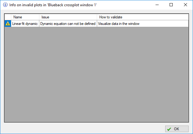 {width="6.197916666666667in" height="4.302083333333333in"}]
[Petrel functions and Blueback equations]{.underline}
[While Blueback Investigator equations and Petrel functions are fundamentally different it is possible to convert Blueback equations to Petrel functions.]
[The Petrel function can be displayed and edited]{.underline} in a scatterplot with the same dimensions as the function.
[To save a Blueback equation as a Petrel function:]
[Right click on the Blueback function in the plot select ]{.underline}[Save to Petrel function]{.underline}
[Right-click on the equation in the control tree and select ]{.underline}[Save to Petrel function]{.underline}
[Right-click on the equation in the legend]
[
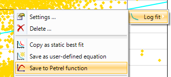 {width="3.6666666666666665in" height="1.6458333333333333in"}]
[
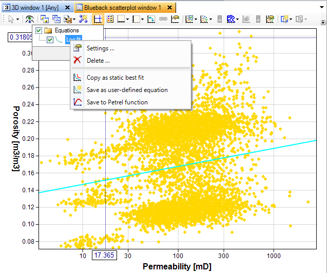 {width="6.197916666666667in" height="5.15625in"}]
[
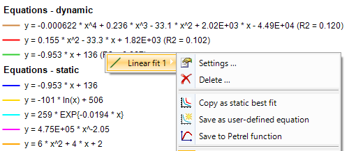 {width="5.208333333333333in" height="2.2604166666666665in"}]
[Coefficient of determination (R2)]{.underline}
[Blueback Investigator calculates the coefficient of determination]{.underline} (R2) to determine the "goodness" of the fit.
[Why do Blueback Investigator and Excel give different values for R2?]{.underline}
[In statistics, there are several different definitions of R2 which are only sometimes equivalent.]
[Microsoft Excel calculates R2 by squaring R (Pearson's correlation coefficient]{.underline}). As such, it is common for Blueback Investigator and Excel to give different values for R2. The wikipedia links further up in the document should help resolve any confusion.
[Why can R2 be negative?]{.underline}
[Reworked from (http://stats.stackexchange.com/questions/12900/when-is-r-squared-negative , user Harvey Motolsky)]
[R2 compares the fit of the chosen model with that of a horizontal straight line. If the chosen model fits worse than a horizontal line, then R2 is negative. ]
[Note that R2 is not always the square of anything, so it can have a negative value without violating any rules of math. R2 is negative only when the chosen model does not follow the trend of the data, so fits worse than a horizontal line.]
[Example - We fit data to a linear regression model constrained so that the Y intercept must equal 1500.]
[
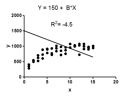 {width="4.427083333333333in" height="3.28125in"}]
[The model makes no sense at all given these data. It is clearly the wrong model, perhaps chosen by accident.]
[The fit of the model (a straight line constrained to go through the point 0,1500) is worse than the fit of a horizontal line. Thus the sum-of-squares from the model (SSreg) is larger than the sum-of-squares from the horizontal line (SStot). R2 is computed as 1 - SSreg/SStot. When SSreg is greater than SStot, that equation computes a negative value for R2.]
[With linear regression with no constraints, R2 must be positive (or zero) and equals the square of the correlation coefficient, r. A negative R2 is only possible with linear regression when either the intercept or the slope are constrained so that the "best-fit" line (given the constraint) fits worse than a horizontal line. With nonlinear regression, the R2 can be negative whenever the best-fit model (given the chosen equation, and its constraints, if any) fits the data worse than a horizontal line.]
[Bottom line: A negative R2 is not a mathematical impossibility or the sign of a computer bug. It simply means that the chosen model (with its constraints) fits the data really poorly.]{.underline}
[Ln or Log10 equations]{.underline}
[Blueback Investigator uses natural logarithms for internal calculations.]
[It is possible to control whether equations are displayed based on natural logarithms (the default) or base 10 logarithms. The drawn equation line does not change, only the equation text will be different. The coefficients will be converted as necessary and any references to Ln and e^ will be replaced to Log and 10^.]
[The text to be displayed is controlled from the equation context menu option as shown below.]
[
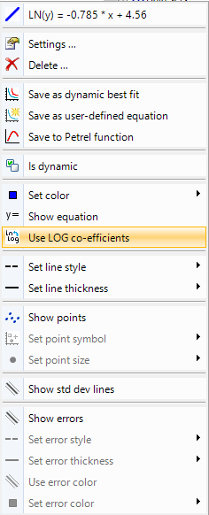 {width="2.4583333333333335in" height="6.0625in"}]
[Distributions]{.underline}
[A distribution is a statistical concept describing the probability function on how values of a variable are distributed. Blueback Investigator supports the creation of distributions from the histogram window.]
[Creating a distribution is simple. Press the add distribution button
 {width="0.2708333333333333in" height="0.21875in"} to access the Add distribution dialog]{.underline}.
[
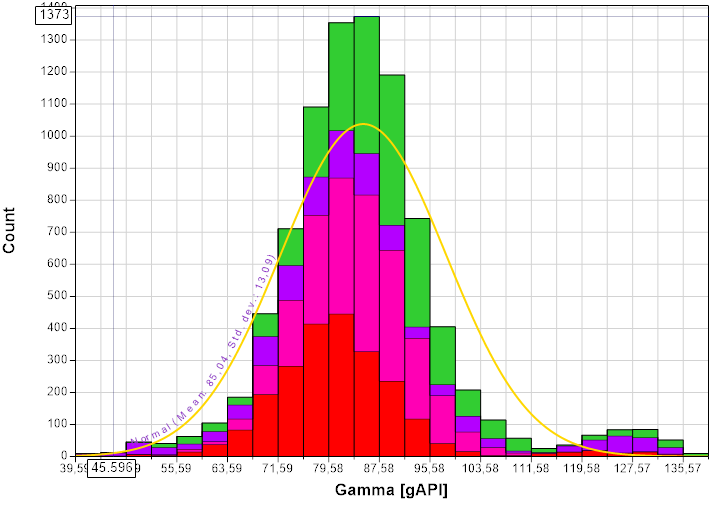 {width="5.333333333333333in" height="3.6979166666666665in"}]{.underline}[
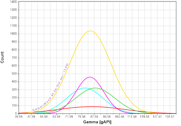 {width="5.3125in" height="3.6875in"}]{.underline}
[Gamma ray normal distribution for a data set with multiple wells. (Left) Normal distribution and distribution for each well (Right)]
[In Blueback Investigator we store this data as a separate domain object called "Distributions". It contains the distribution type, if it is dynamic or not, the standard deviation, number of points, the mean plus the min/max of the value range: ]
[
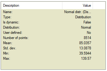 {width="3.6458333333333335in" height="2.4270833333333335in"}]
[The objects are available from the Windows control tree.]
[
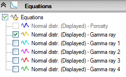 {width="2.71875in" height="1.6666666666666667in"}]
[A distribution can be either static or dynamic. A dynamic distribution will update to whatever data that is displayed in the window. A static distribution will create the distribution from the displayed data and lock it down into a data object that cannot be changed. ]
[Blueback Investigator supports different distribution types:]
[Normal]{.underline} (Gaussian)
[A distribution can be drawn in any plot space in which it is valid.]
[A distribution can be used as input to the "Data reshaper]{.underline}" tool.
[Add distribution]{.underline}
[
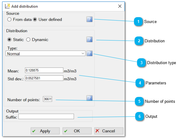 {width="6.135416666666667in" height="4.71875in"}]
[
{width="0.4166666666666667in" height="0.4166666666666667in"}]{.underline}[Source]{.underline}[
 {width="3.1354166666666665in" height="0.5208333333333334in"}]
[Choose the distribution data source.]
[Determines if the distribution parameters are estimated based on the selected data in the histogram window or explicitly specified by the user. Note that the default values of the parameters when User defined mode is selected will be calculated based on the presented data. The selection of the source determines if the parameters below are displayed or not. ]
[
{width="0.4166666666666667in" height="0.4166666666666667in"}]{.underline}[Distribution]{.underline}[
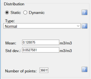 {width="3.1875in" height="2.7604166666666665in"}]
[Select the distribution type and its behavior. ]
[Three distributions are supported:]
[1. Normal (Guassian): If set from data, the distribution is based on the mean and standard deviation of the data. Otherwise, can be specified explicitly.]
[2. Log normal: If set from data, the distribution parameters Mu and Sigma are calculated from the mean and standard deviation. Otherwise, specified explicitly by the user.]
[3. Continuous uniform: If set from data, the lower and upper bound are calculated from the data range. Otherwise, specified explicitly by the user.]
[The Static/Dynamic mode set the behavior of the plot. A static distribution will retain its parameters while a dynamic distribution will update when the underlying data changes.]
[Number of points is used to scale the distribution curve. If the data source is from data or the mode is dynamic, number of points will be the total number of displayed data. Otherwise, it's user defined.]
[ ]
[
{width="0.4166666666666667in" height="0.4166666666666667in"}]{.underline}[Distribution type]{.underline}[
 {width="3.03125in" height="0.4166666666666667in"}]
[Select the distribution type]
[
{width="0.4166666666666667in" height="0.4166666666666667in"}]{.underline}[Parameters]{.underline}[
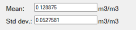 {width="2.8125in" height="0.6354166666666666in"}]
[The parameters section will be present only if user defined source is selected. ]
[
{width="0.4166666666666667in" height="0.4166666666666667in"}]{.underline}[Number of points]{.underline}[
 {width="1.8020833333333333in" height="0.3125in"}]
[Number of points used in creating the distribution curve. This setting is not available if the data source is from the data or if the mode is dynamic.]
[
{width="0.4166666666666667in" height="0.4166666666666667in"}]{.underline}[Output]{.underline}[
 {width="2.53125in" height="0.5625in"}]
[Optional suffix that can be added to the distribution name]
[Display, edit and create Petrel function]{.underline}
[Petrel functions can be created, displayed and edited in the scatterplot and crossplot windows.]
[
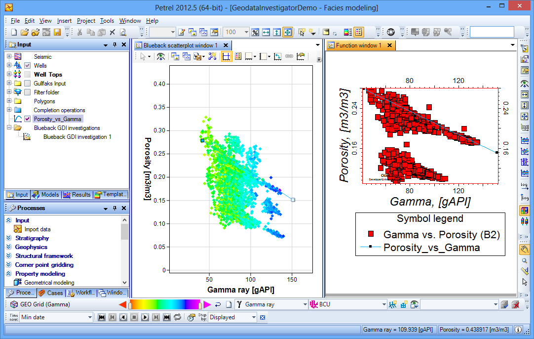 {width="6.197916666666667in" height="3.9270833333333335in"}]
[The Y and X axis need to be set up in the same way as in the function window for the Petrel function to plot in the Blueback Investigator windows.]
[Points can be added to the function]
[
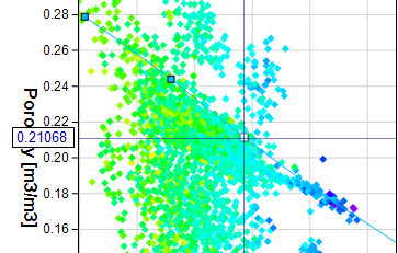 {width="3.78125in" height="2.40625in"}]
[A spline can be applied by right-clicking on the line]
[
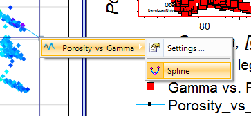 {width="3.78125in" height="1.75in"}]
[Petrel functions with same template as X and Y dimension]{.underline}
[Blueback Investigator supports using the same template as input for different dimensions. For Petrel Functions this means that you can have a plot where the X and Y dimensions are using the same template. In these special cases, a swap axis will not transform the displayed function, since it is impossible to distinguish the two templates.]
[Petrel functions with Ln data]
[While Blueback Investigator supports equations with logarithmic data and displays them correctly; the same cannot be said for Petrel. As such, if a logarithmic equation is exported to a Petrel function it is often necessary to manually set the Log property in the function and when displaying in the Petrel function window.]
[Annotations]{.underline}
[In order to mark points of interest and comment on the plotted data, annotations can be added to the plots.]
[
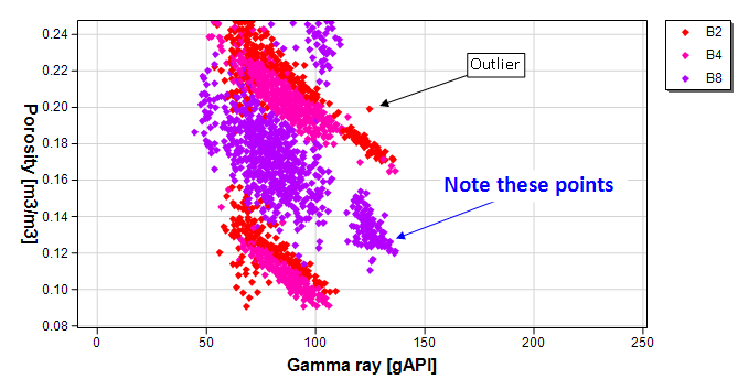 {width="6.197916666666667in" height="3.2708333333333335in"}]
[Annotations are ]{.underline}[stuck]{.underline}[ to the data so will continue to point to the same place as plots are scrolled and zoomed. Annotations are also specific to the data template space in which they have been created. This means that if the axis data selections are changed (via the
 {width="0.8229166666666666in" height="0.20833333333333334in"} toolbar buttons) then the annotation will no longer appear. For example, the above scatterplot displays two annotations on a gamma ray v porosity plot. If the axes are swapped such that the plot now displays porosity v gamma ray the annotations will not be displayed. The same is true for histograms when the y-axis is changed between count and percentage.]
[Annotation settings and style can be controlled from the Blueback investigation. Most style settings are also available from the context menu inside of the plot:]
[
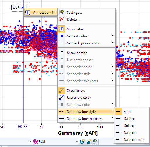 {width="5.34375in" height="5.239583333333333in"}]
[X, Y, Time and Depth plots]{.underline}
[Blueback Investigator supports special spatial dimensions]{.underline} for plotting data in X, Y, depth or time.
[For well data, if a time depth relationship is defined, then Blueback Investigator will automatically use the T/D relationship as input to the spatial dimensions. This means you can add both Time and Depth as a dimension. For all other data types you need to add the depth or time attribute as a separate dimension by selecting the attribute specifically.]
[
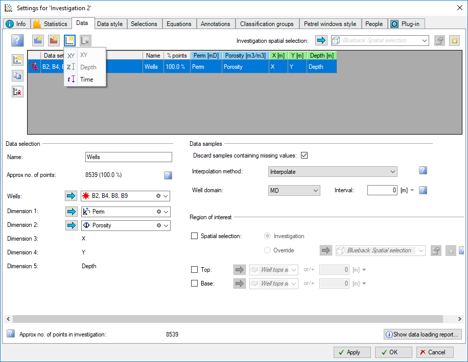 {width="6.197916666666667in" height="4.802083333333333in"}]
[Add spatial dimensions to your investigation]{.underline}
[A matrix window with spatial dimensions could look something like this:]
[
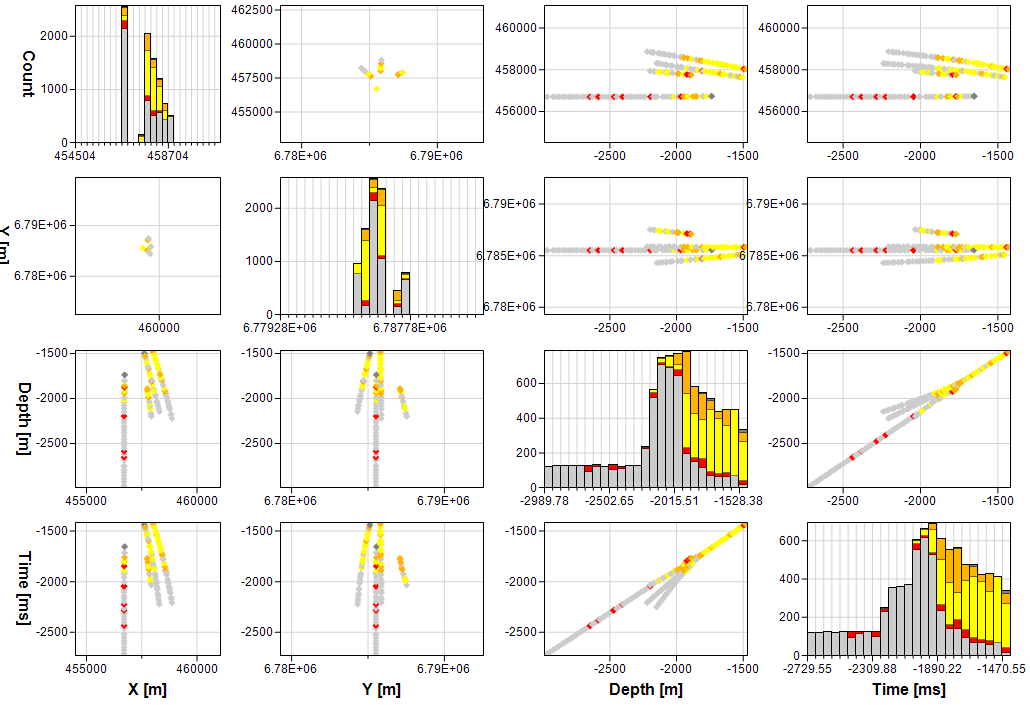 {width="6.197916666666667in" height="4.239583333333333in"}]
[Measure distance]{.underline}
[In spatial XY plots the Measure distance option is available:]
[
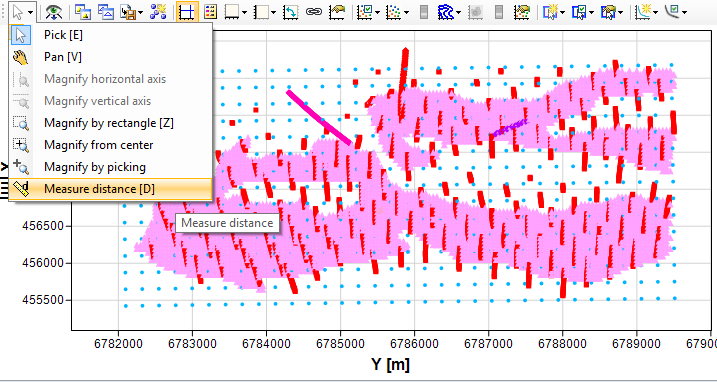 {width="6.197916666666667in" height="3.3020833333333335in"}]
[Dragging the Measure distance tool over the plot displays the distance:]
[
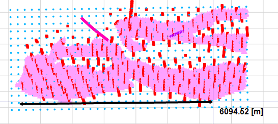 {width="5.6875in" height="2.5416666666666665in"}]
[Linked views]{.underline}
[A single Blueback investigation can act as the source data for any number of windows. ]
[Linked views allow the user to ensure that the same ranges of data are displayed in each of the windows viewing the same Blueback investigation. Note that only the axis ranges are linked; the data selections. visibility and other settings are not linked.]
[Linking of views is achieved using the ]{.underline}[Link axis view]{.underline}[ button (
 {width="0.20833333333333334in" height="0.20833333333333334in"}) which can be found in the window toolbar. The user can then select which window they wish to link to. Once the link has been established, the window will update to match the axes ranges of the selected window. Note that the selected window does not need to display the same axes to link the views.]
[Linked views allows the user to have the full functionality of the histogram and scatterplot windows but display the Blueback investigation in a similar setup to a crossplot window.]
[The example below shows a permeability vs gamma ray scatterplot colored by porosity linked to a histogram for each template. Notice how the data axis range is the same for the scatterplot dimensions as in the corresponding histogram windows.]
[
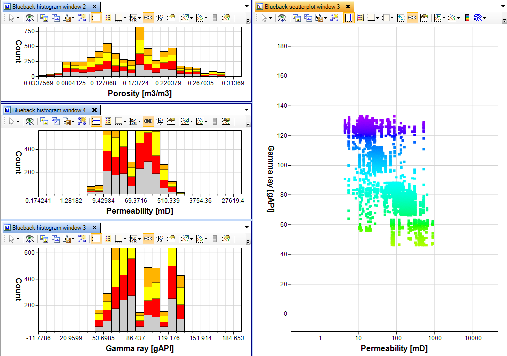 {width="6.197916666666667in" height="4.354166666666667in"}]
[Picked points - visualization]{.underline}
[When picking a point in the crossplot or matrix windows, a point get highlighted with a +:]
[
 {width="1.2395833333333333in" height="1.0833333333333333in"}]
[If the same investigation is displayed in many windows the point will be highlighted with a + or a bold line in the parallel coordinates window.]
[
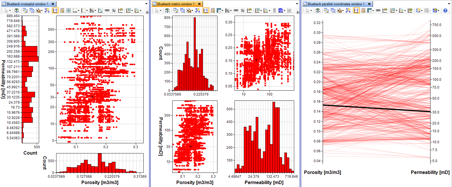 {width="6.197916666666667in" height="2.5520833333333335in"}]
[Relating conceptual and real world space]{.underline}
[Blueback Investigator features two ways of translating what you see in your conceptual plot space into real world 3D space.]
[Display investigation in Petrel window]{.underline}
[The user can now display investigations containing spatial dimensions in the following Petrel windows.]
[
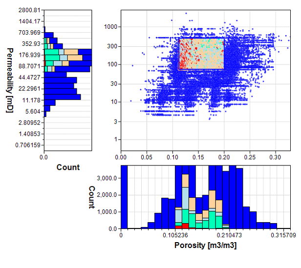 {width="5.708333333333333in" height="5.083333333333333in"}]
[Set up your selection in the investigation window.]
[
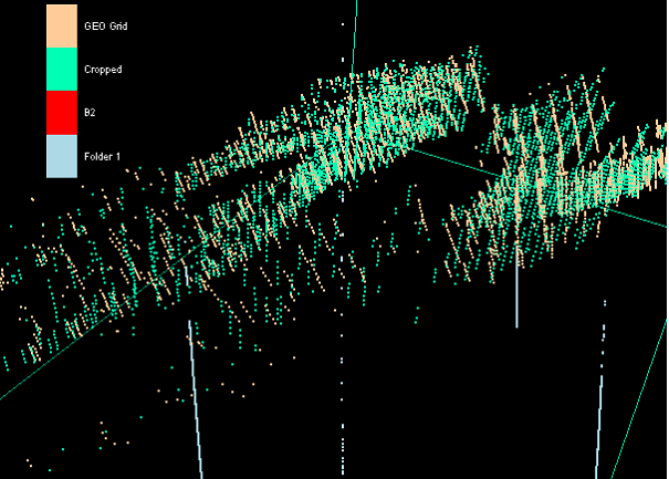 {width="6.197916666666667in" height="4.427083333333333in"}]
[Create indicator objects]{.underline}
[Another way of exporting data from the conceptual plot space into real world coordinates is to use the indicator logs, indicator seismic and indicator model properties.]
[
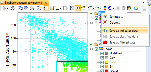 {width="6.197916666666667in" height="2.96875in"}]
[Save the indicator objects from the context menu of the relevant folder/data in the "ontrol data points"tree. ]
[
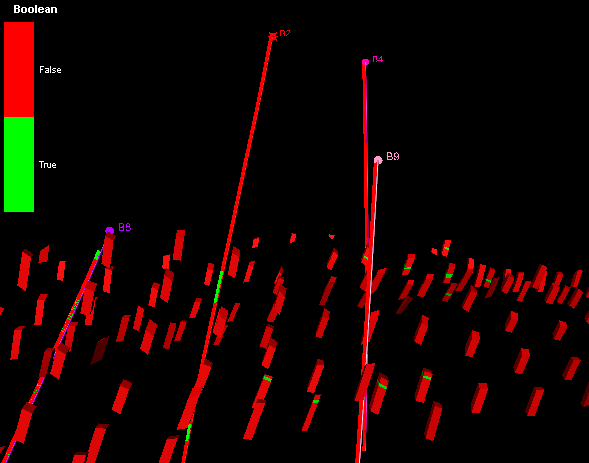 {width="6.135416666666667in" height="4.822916666666667in"}]
[The result is one indicator object per data type displayed in Blueback Investigator. The "rue"value is the unrestricted values based on the active visible data as defined in the plot window.]
[Export options]{.underline}
[Blueback Investigator features different ways of saving the data you are displaying in an investigation.]
[Export to spreadsheet]{.underline}
[This option exports the entire view or the active points based on one or more selections. The export also honors the window data points selection.]
[
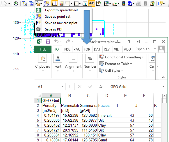 {width="6.052083333333333in" height="5.09375in"}]
[Export the active displayed points into a spreadsheet for further analysis!]
[Save as point set]{.underline}
[Create a Petrel point set based on the active/visible data in the current plot. All the dimensions present in the investigation will be exported with the correct template. The data attribute is a discrete attribute that contains information about where the data came from.]
[
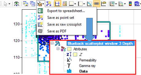 {width="4.78125in" height="2.53125in"}]
[Save as raw crossplot]{.underline}
[Create a Petrel Raw crossplot object based on the active/visible data in the current plot. The displayed dimensions will be included in the plot. The raw cross plot can be displayed in the function window and used in property modeling workflows.]
[
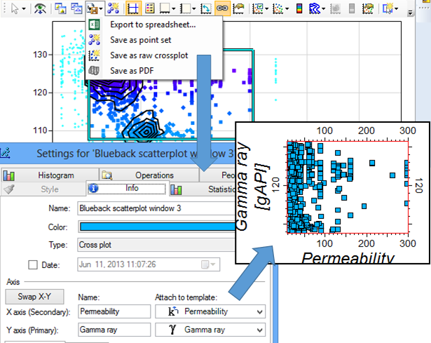 {width="6.197916666666667in" height="4.927083333333333in"}]
[Save as PDF]{.underline}
[If contours are displayed, you can export the contour data as probability density functions. The PDF's are stored as surfaces in the Input tree. The PDF can be used as input to Blueback Rock physics]
[
 {width="2.4270833333333335in" height="0.9375in"}]
[The PDF can be displayed in the 3D window.]
[
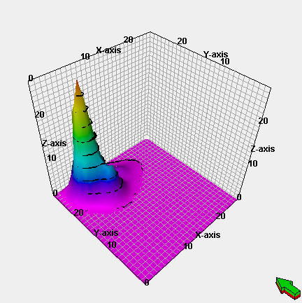 {width="4.5in" height="4.510416666666667in"}]
[Export to invpy]{.underline}
[<TODO>: Insert description text here... And don't forget to add keyword for this topic]
[Copy window to emf and bitmap]{.underline}
[In Blueback Investigator all windows can be grabbed by using the ]{.underline}[Copy bitmap]{.underline}[ or ]{.underline}[Copy enhanced metafile]{.underline}[ options (
 {width="0.4791666666666667in" height="0.25in"}). The data is put on the clipboard and can be used in other applications.]
[The Blueback Investigator enhanced metafile contains vector information only and is great for printing and resizing your data. This is the recommended copy format for any printed material that is to be made from Blueback Investigator.]
[
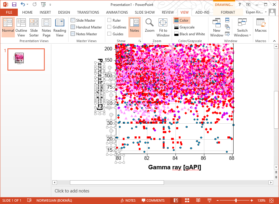 {width="6.197916666666667in" height="4.53125in"}]
[Expanding viewports]{.underline}
[A window can contain several viewports. In Blueback Investigator double clicking the void space in a combined window expands viewport to cover the full window extents.]
[
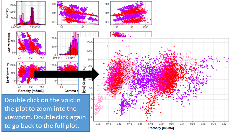 {width="6.197916666666667in" height="3.5729166666666665in"}]
[An expanded window will get [Expanded] added to the Window title:]
[
 {width="3.1875in" height="1.7083333333333333in"}]
[Incomplete investigations]{.underline}
[An investigation can be incomplete for two reasons:]
[Missing dimensions]{.underline}
[The datasets used in an investigation can contain missing dimensions. For instance wells may have time and depth defined, but seismic datasets/models do not support a dataset with both combined. Alternatively, you can have Gamma ray defined in your logs but not in the model. ]
[In Blueback Investigator this will be highlighted to the user in different ways.]
[
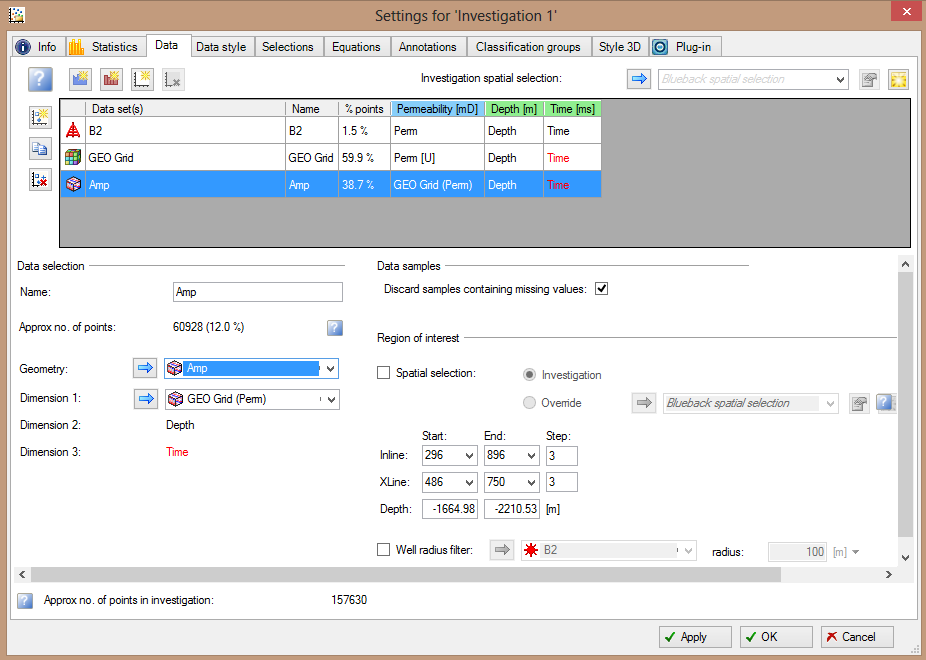 {width="6.197916666666667in" height="4.416666666666667in"}]
[The investigation dialog will highlight missing spatial dimensions in red. The investigation is still valid.]
[Missing data is highlighted in the window with a Yellow border:]
[
 {width="5.1875in" height="4.302083333333333in"}]
[In the image above, only one dimension is defined.]
[If one of many datasets has a missing dimension, a yellow line is also displayed. The complete and valid dimensions will be displayed. The invalid dataset will be listed in the legend:]
[
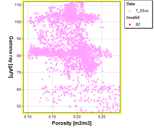 {width="5.1875in" height="4.302083333333333in"}]
[If plot is highlighted with a yellow border, this button will be enabled in the toolbar:
{width="0.25in" height="0.23958333333333334in"} Click the button to open info dialog with information regarding the invalid plot(s).][
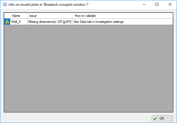 {width="6.197916666666667in" height="4.302083333333333in"}]
[Missing values]{.underline}
[The data selection dialog contains an option for each dataset that allows the user to control how Blueback Investigator manages samples containing missing values.]
[The default behavior is to discard samples that contain missing values.]
[The user can choose not to discard these samples using the following control:]
[
 {width="4.052083333333333in" height="0.6354166666666666in"}]
[Toggling to not discard samples containing missing values will load all the data into Blueback Investigator and the statistics for each dimension will be those expected. However, where multiple dimensions are needed (eg scatterplot), only samples containing values in all the required dimensions will be displayed.]
[This option is of particular importance during data selection for well and table data (see Well logs]{.underline} and [Table data]{.underline})
[Units]{.underline}
[Display unit handling]{.underline}
[When setting up dimensions in the investigation the units defined in the corresponding template are used as the Dimension units.]
[Note: Any changes made to the Dimension tab units have direct effect on what is displayed. Input data values are not changed. Please use with caution in the analysis.]{.underline}
[Example]{.underline}
[Porosity data is added to the investigation. This has the unit mD.]
[
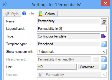 {width="3.9583333333333335in" height="2.8229166666666665in"}]
[When added to the investigation the mD unit is used as the dimension unit, but can be changed at any time:]
[
 {width="2.78125in" height="1.4895833333333333in"}]
[Changing the units will not transform the input data values, only the displayed units.]
[Change the display units in the window]{.underline}
[When displaying data in a Blueback Investigator window, the default display unit is what is defined in the Data selection Dimension tab]{.underline}.
[The user can temporarily change the display unit by right-clicking on the dimension axis. This reveals the ]{.underline}[Display unit]{.underline}[ option:]
[
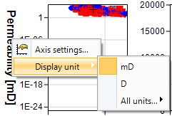 {width="2.5104166666666665in" height="1.6979166666666667in"}]
[Memory management]{.underline}
[The Blueback investigation has mechanisms that lets the user unload and load points into memory.]
[Manage investigations]{.underline}
[Memory used by individual Blueback Investigations can be managed. See Load and unload points]{.underline} for more information.
[Free memory]{.underline}
[Blueback Investigator is hooked up to the Petrel Free memory mechanism. This means that investigations are unloaded from memory when the Free memory button is pressed.]
[
 {width="4.333333333333333in" height="1.0625in"}]
[Tuning the investigation performance]{.underline}
[Petrel loads data in several different ways. Blueback Investigator makes use of the Ocean APIs to read the data it needs from the open Petrel project. This means that Blueback Investigator's perceived performance is highly influenced by how fast Petrel can provide Blueback Investigator the data it requests. ]
[ ]
[This guide gives some ideas on how perceived performance can be improved, examples of memory usage and a quick explanation on how an investigation reads and stores data. Many other things also influence performance such as hardware, project size and project location. These are not widely discussed in this section.]
[ ]
[Data decimation]{.underline}
[When the user creates a Blueback investigation, the requested dataset is read from Ocean and recreated in the investigation data structure. The duplicated data structures are needed to maintain performance and to give users access to many data types in one go.]
[ ]
[By default, the investigation is decimated when seismic and model datasets are added to it. This is done to ensure performance and reduces the initial time it takes to display data in the windows.]
[ ]
[The Blueback Investigator data engine works with point data in the specifically defined Blueback Investigator data structure. The more points that are loaded into the investigation the longer it takes to load. This is why it is important to keep a track on the number of points in the investigation, both at a dataset level, but also for the whole investigation. This decimation is done by applying a region of interest or general decimation (Valid for models and seismic).]
[ ]
[Datasets over 100 000 points are automatically decimated so it will contain less than 100 000 points when added to the investigation. This can be changed at a later stage, and for a full data export, all points should be considered. For each dataset in the investigation how many points are loaded and the percentage of the total dataset points that are loaded is reported to the user.]
[ ]
[Once added to the investigation each dataset will report how much of the data that has been loaded, as a percentage of the total number of points. The total number of points loaded to the investigation is displayed on the Data selection tab. If you have many datasets in the investigation then monitor the total number of points closely before visualizing the data. ]
[ ]
[Visualization performance is tied to the machine specifications. This is not covered in this section. It should be tested so that the user can get an understanding on how point rendering affects the Blueback Investigator window performance.]
[ ]
[Example]{.underline}[ - 12.0% of the Amp dataset is loaded, based on the ]{.underline}[Region of interest]{.underline}[ step decimation settings. In addition Well B2 and Model GEO Grid is loaded. The investigation has a total of 157630 points (1.5% B2, 59.9% GEO grid and 38.7% Amp):]
[ ]
[
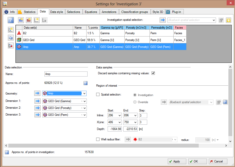 {width="6.197916666666667in" height="4.40625in"}]
[ ]
[To guide the user when the investigation may become too large, Blueback Investigator highlights in red text the total number of points when it is over 1 000 000 for the investigation or per dataset. ]
[ ]
[Example]{.underline}[ - GEO grid loads 24.3% of the dataset; over 1 million points. This makes the dataset ]{.underline}[Approx no. of points]{.underline}[ and the total ]{.underline}[Approx. number of points]{.underline}[ text red to indicate that perceived performance might be affected:]
[ ]
[
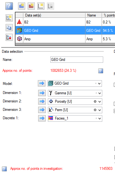 {width="3.8541666666666665in" height="5.739583333333333in"}]
[ ]
[NB The 1,000,000 point limit is just provided as a guide. The system may work fine with more points.]{.underline}
[ ]
[ ]
[Memory used by investigation]{.underline}
[The total memory used by the investigation can be found in the statistics tab in the investigation dialog. This gives an indication on how much memory the investigation uses:]
[ ]
[
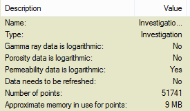 {width="2.8645833333333335in" height="1.6770833333333333in"}]
[ ]
[However, to the user this may not add up if you compare with the total memory usage of Petrel, before and after the investigation was loaded. This is because the total memory usage is a factor of many things. The Petrel seismic cache, the size of the Petrel project, number of investigations loaded and the number of windows in use with data displayed.]
[Unload data from the investigation]{.underline}
[Data loaded into investigations can be unloaded from memory. This can be done by right-clicking the investigation and selecting ]{.underline}[Unload all points]{.underline}[:]
[ ]
[
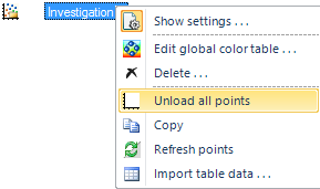 {width="3.0104166666666665in" height="1.78125in"}]
[ ]
[If you have many investigations loaded, this needs to be repeated for each investigation.]
[ ]
[Use of seismic data]{.underline}
[The Petrel seismic cache should be set large enough so it can contain all the seismic data that is to be used in the investigation. (Factor in all the dimensions when deciding upon the size of the cache.) Failing to do this might force the system to start reading data from disk, thus lowering performance.]
[Free memory]{.underline}
[Memory consumed by Blueback Investigator can be removed by using the Petrel ]{.underline}[Free memory]{.underline}[ option. Select ]{.underline}[File]{.underline}[->]{.underline}[Tools]{.underline}[->]{.underline}[Free memory]{.underline}[ or interact with the ]{.underline}[RAM monitor]{.underline}[ to free the Petrel memory.]
[
 {width="2.6875in" height="0.8020833333333334in"}]
[NB Free memory will only free all Blueback investigations not in use by any displayed windows. Please close all windows to clear all Blueback Investigator data from the Petrel memory.]{.underline}
[Further reading]{.underline}
[Please look in the Petrel user guide for more help about how to optimize your Petrel environment:]
[·Home / Geophysics / Seismic Basic and Visualization / Data Management / Seismic data - Memory management]
[·Home / Environment Setup / Configuring Petrel / Optimizing Memory Usage]
[·Home / Environment Setup / Configuring Petrel / Virtual Memory]
[Load and unload points]{.underline}
[The Blueback investigation has mechanisms that lets the user unload and load points into memory.]
[
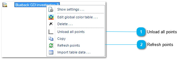 {width="6.052083333333333in" height="2.0104166666666665in"}]
[
{width="0.4166666666666667in" height="0.4166666666666667in"}]{.underline}[Unload all points]{.underline}[
 {width="1.90625in" height="0.2916666666666667in"}]
[This removes the loaded points from the Petrel memory]
[
{width="0.4166666666666667in" height="0.4166666666666667in"}]{.underline}[Refresh points]{.underline}[
 {width="1.875in" height="0.2916666666666667in"}]
[This loads the investigation contents into memory or refreshes the already loaded investigation]
[Interpolation options]{.underline}
[Blueback Investigator supports the following different interpolation options for well data:]
- All well logs will be resampled to a common sampling interval. This is the default setting.
- Well logs values will only be accepted if they match the sampling of the well log in dimension 1. For some log types, e.g. core logs, the nature of the data is discrete, so interpolation may introduce incorrect results.
- No interpolation will be performed. Well logs values will only be accepted if they match the sampling of the selected dimension. For some log types, e.g. core logs, the nature of the data is discrete, so interpolation may introduce incorrect results.
- [None]
This will cause Blueback Investigator to not discard invalid samples and will load the raw well log data with no interpolation. All the statistics for each log will match Petrel statistics but if the different logs are not sampled at the same MD values it is possible for no points to be displayed in the scatterplot.
[The details of each option are explained in for each separate helps pages. For each interpolation option, the same raw data is used and the impact in the data with Blueback Investigator can be seen.,]
[Interpolate]{.underline}
[When interpolation is performed the all ]{.underline}[raw]{.underline}[ data from all the dimensions is interpolated to a consistent sample rate before being loaded into Blueback Investigator.]
[This option allows the user to investigate continuous data that may have been recorded at different sample rates.]
[
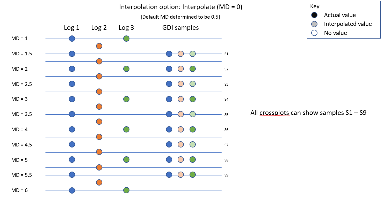 {width="6.197916666666667in" height="3.4583333333333335in"}]
[Sampling from Dimension (Interpolate other dimensions)]{.underline}
[When sampling from dimension (interpolate other dimensions) is selected the ]{.underline}[raw]{.underline}[ data from the selected dimension is loaded into Blueback Investigator. Data from the other dimensions will be interpolated so that it co-locates with the sampling from selected dimension. The user can select the dimension within the dataset that defines the sampling to be used.]
[This option allows the user to investigate the relationships between core log data and log data.]
[
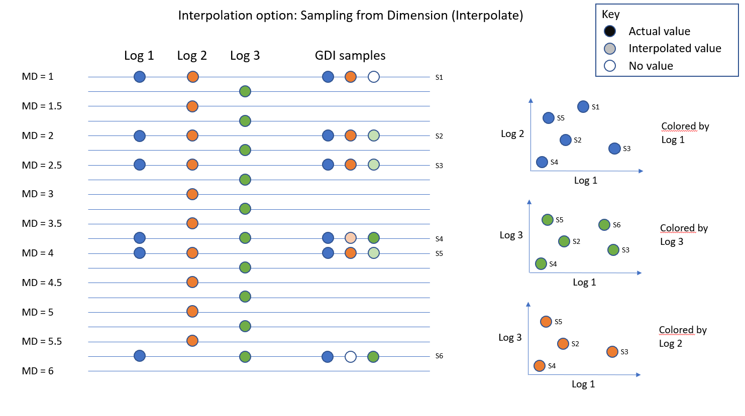 {width="6.197916666666667in" height="3.4583333333333335in"}]
[Sampling from Dimension (No interpolation)]{.underline}
[When sampling from dimension with no interpolation is selected the ]{.underline}[raw]{.underline}[ data from the selected dimension is loaded into Blueback Investigator. Data is only loaded for the other dimensions when the data co-locates with the selected dimension. The user can select the dimensions within the dataset define from which sampling is to be used.]
[.]
[This option allows the user to investigate the data that is exists at known samples. but it can lead to confusion if the data for each dimension is not consistently sampled or is missing.]
[
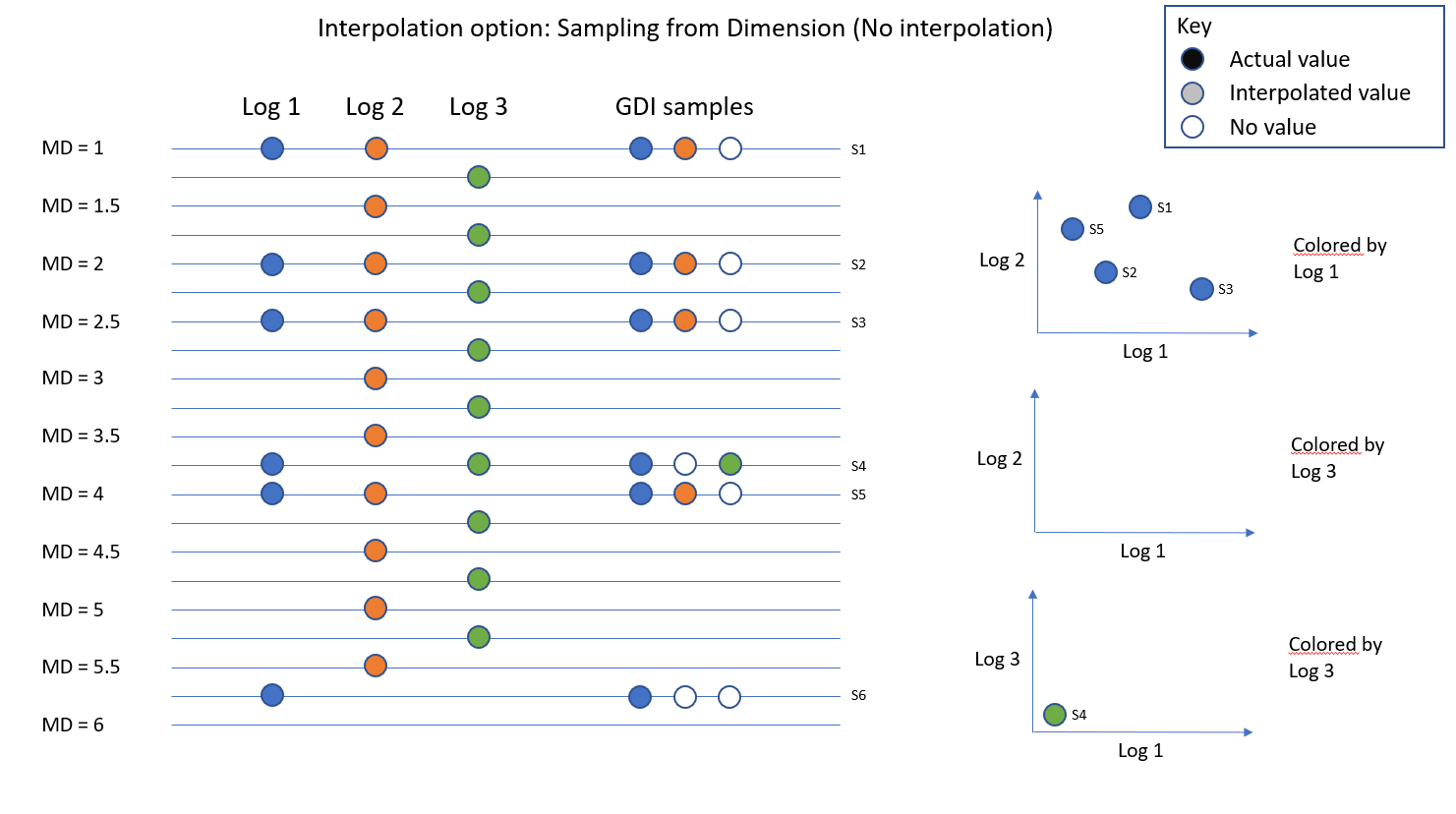 {width="6.197916666666667in" height="3.4583333333333335in"}]
[No interpolation]{.underline}
[When no interpolation is performed the ]{.underline}[raw]{.underline}[ data is loaded into Blueback Investigator. When using the None option it is important that the user also selects to not discard samples containing missing values (see here]{.underline}).
[This option allows the user to investigate the raw data but it can lead to confusion if the data for each dimension is not consistently sampled or is missing.]
[
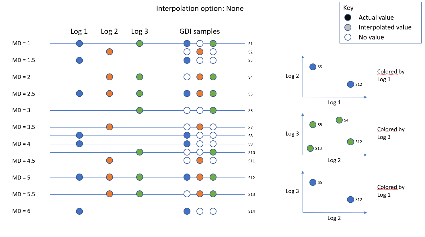 {width="6.197916666666667in" height="3.4583333333333335in"}]
[Overplot data and decimation]{.underline}
[It is possible to control the additional plotting options for scatterplots via the Show data]{.underline} (
 {width="0.20833333333333334in" height="0.19791666666666666in"}) dropdown option. The options described below were implemented to improve render performance. The default options replicate the rendering used in previous versions of Blueback Investigator.
[Note: These options should be changed with caution. On large datasets, these options can result in significantly more data being rendered which may cause performance problems.]{.underline}
[Decimation]
[Defaults to on. ]
[When decimation is on, the appearance options are used to determine the size of the smallest symbol to be rendered. This data is then decimated so that symbols are only drawn when more than half a shape size apart. This reduces the number of symbols rendered (when most samples are close to each other) and makes very little difference to the rendered image.]
[The image on the left has decimation applied, the image on the right does not.]
[
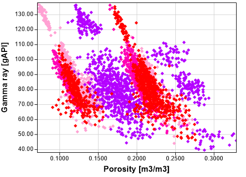 {width="5.177083333333333in" height="3.7291666666666665in"}
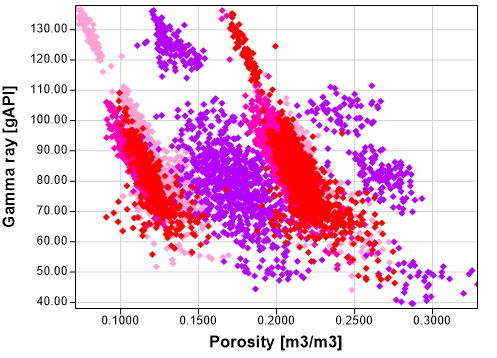 {width="5.177083333333333in" height="3.7291666666666665in"}]
[Overplotting of data]{.underline}
[Defaults to off.]
[When overplotting is off, a single symbol is drawn in each pixel. If more than 1 sample should be rendered at a pixel then symbol from the dataset will the highest priority will be drawn. This reduces the number of symbols rendered (when symbols are the same shape there is no point rendering multiple at the same location as only the symbol from the dataset will the highest priority will be visible). However, if different symbols are used then it will not be clear that the lower priority dataset was data are some locations.]
[When overplotting is on, all symbols are drawn. This allows lower priority datasets to be shown behind higher priority allowing differences to be viewed.]
[Note: Toggling overplot also changes decimation. When overplotting is on, then decimation is turned off to ensure all data is rendered.]{.underline}
[The image on the left has overplotting off, the image on the right has overplotting on. The datasets are identical but using different appearances.]
[
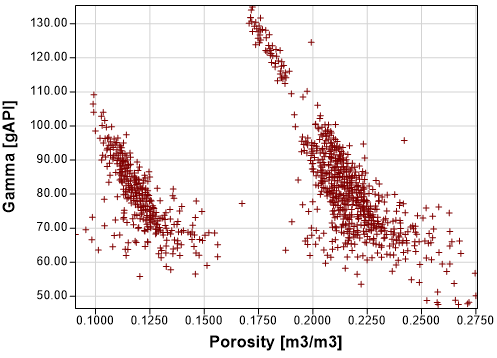 {width="5.177083333333333in" height="3.7291666666666665in"}
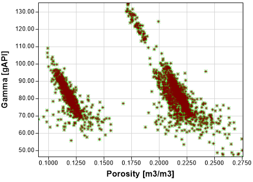 {width="5.177083333333333in" height="3.7291666666666665in"}]
[Data selection]{.underline}
[The Blueback Investigator requires a special collection of data to be set up, called an ]{.underline}[Investigation]{.underline}[, to be defined before the functionality can be used. ]
[All data types are tied together with dimensions]{.underline} that are based on Petrel templates. This allows many different data types to be compared and analyzed.
[The dimension are shown as columns with colored headers and are added/removed using the buttons along the top of the table.]
[Blue for continuous dimensions]
[Green for spatial dimensions]
[Red for discrete dimensions]
[The datasets are shown as rows in the table and are added/removed using the buttons to the left of the table. Each row in the table represents a dataset. The data type of the dataset is indicated by the image at the start of each row.]
[The controls below the table are dependent on what the user has selected. Clicking anywhere in a row will cause the controls for that dataset]{.underline} to be displayed. Clicking on a colored column header will cause the controls below the table to change to the [dimension]{.underline} controls.
[An investigation spatial selection]{.underline} can also be selected which can be referenced by many datasets.
[A data loading report]{.underline} can be generated on this tab.
[
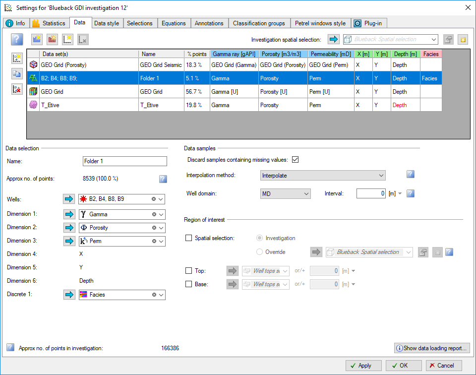 {width="6.197916666666667in" height="4.875in"}]
[Multi-select]{.underline}
[Datasets and dimensions can be quickly added using multi-selection (where supported). ]
[This feature allows the user to select a number of datasets or properties in a single dropbox. When the dropbox content is accepted additional datasets or dimensions will be added to the investigation as necessary based on the users selections. This significantly reduces the number of clicks necessary to define an investigation.]
[Multi-select is support for the majority of datasets, continuous properties and discrete properties.]
[For example, if the user want to add a number of surface datasets they could select the datasets as shown in the left image and this would create many datasets in the investigation as shown in the right image.]
[
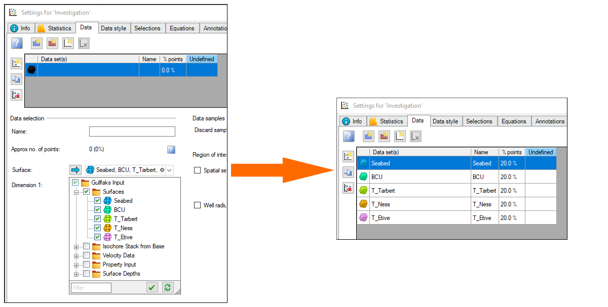 {width="6.197916666666667in" height="3.125in"}]
[Investigation spatial selection]{.underline}
[The investigation spatial selection allows a single spatial selection to be easily shared across multiple datasets within the investigation.]
[Each dataset within the investigation can choose to apply a spatial selection and can either refer to the investigation spatial selection of provide a spatial selection specific to the dataset.]
[
 {width="6.197916666666667in" height="1.0416666666666667in"}]
[
{width="0.4166666666666667in" height="0.4166666666666667in"}]{.underline}[Select investigation spatial selection]{.underline}[
 {width="4.541666666666667in" height="0.2604166666666667in"}]
[This allows the user to select a Blueback spatial selection that can be used by the investigation.]
[
{width="0.4166666666666667in" height="0.4166666666666667in"}]{.underline}[Show spatial selection settings]{.underline}[
 {width="0.3333333333333333in" height="0.3333333333333333in"}]
[Opens the settings dialog for the selected spatial selection]
[
{width="0.4166666666666667in" height="0.4166666666666667in"}]{.underline}[New spatial selection]{.underline}[
 {width="0.34375in" height="0.34375in"}]
[Creates a new Blueback spatial selection and selects it.]
[Datasets]{.underline}
[The Data tab in the Blueback investigation settings dialog allows multiple data types to be selected for plotting in a single window. It supports many data types. Additionally, data can be pasted or manually entered and edited as ]{.underline}[Table data]{.underline}[, allowing any type of data from any source to be plotted alongside Petrel data.]
[
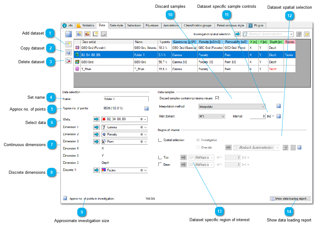 {width="6.197916666666667in" height="4.458333333333333in"}]
[
{width="0.4166666666666667in" height="0.4166666666666667in"}]{.underline}[Add dataset]{.underline}[
 {width="0.25in" height="0.3020833333333333in"}]
[Adds data to the investigation. Pressing the button reveals a drop down menu with all the supported data types:]
[
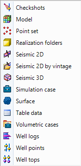 {width="1.75in" height="3.5520833333333335in"}]
[Once selected a new undefined dataset is created in the investigation and data is displayed in the table and in the data selection and region of interest part of the dialog.]
[
{width="0.4166666666666667in" height="0.4166666666666667in"}]{.underline}[Copy dataset]{.underline}[
 {width="0.34375in" height="0.3645833333333333in"}]
[Creates a copy of the currently selected dataset and add this to the investigation.]
[
{width="0.4166666666666667in" height="0.4166666666666667in"}]{.underline}[Delete dataset]{.underline}[
 {width="0.34375in" height="0.3645833333333333in"}]
[Delete the selected dataset row]
[
{width="0.4166666666666667in" height="0.4166666666666667in"}]{.underline}[Set name]{.underline}[
 {width="3.03125in" height="0.2708333333333333in"}]
[Define dataset name.]
[
{width="0.4166666666666667in" height="0.4166666666666667in"}]{.underline}[Approx no. of points]{.underline}[
 {width="3.0416666666666665in" height="0.28125in"}]
[
{width="0.4166666666666667in" height="0.4166666666666667in"}]{.underline}[Select data]{.underline}[
 {width="3.0104166666666665in" height="0.3645833333333333in"}]
[Area for selection of data to be included in the dataset.]
[
{width="0.4166666666666667in" height="0.4166666666666667in"}]{.underline}[Continuous dimensions]{.underline}[
 {width="3.03125in" height="1.3854166666666667in"}]
[Area where continuous dimensions are added. ]
[To help find the desired template, type text in the filter field at the bottom of the drop down.]
[
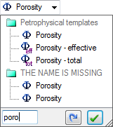 {width="1.6770833333333333in" height="1.8854166666666667in"}]
[
{width="0.4166666666666667in" height="0.4166666666666667in"}]{.underline}[Discrete dimensions]{.underline}[
 {width="3.1041666666666665in" height="0.3541666666666667in"}]
[Area where discrete dimensions are added. ]
[
{width="0.4166666666666667in" height="0.4166666666666667in"}]{.underline}[Approximate investigation size]{.underline}[
 {width="3.2083333333333335in" height="0.2604166666666667in"}]
[Shows the approximate number of points in the entire investigation. It is the sum of all the approximate point numbers for all the investigation datasets.]
[
{width="0.4166666666666667in" height="0.4166666666666667in"}]{.underline}[Discard samples]{.underline}[
 {width="2.1770833333333335in" height="0.2708333333333333in"}]
[Define how this dataset should deal with samples containing missing values.]
[SeeMissing values]{.underline} for more information.
[
{width="0.4166666666666667in" height="0.4166666666666667in"}]{.underline}[Dataset specific sample controls]{.underline}[Any controls a specific dataset might have for handling samples will appear here.]
[
{width="0.4166666666666667in" height="0.4166666666666667in"}]{.underline}[Dataset spatial selection]{.underline}[
 {width="4.947916666666667in" height="0.9270833333333334in"}]
[Defines whether the dataset is constrained by a spatial selection. Use this to control if the investigation spatial selection is to be used to constrain this dataset or if a different spatial selection should be used.]
[
{width="0.4166666666666667in" height="0.4166666666666667in"}]{.underline}[Dataset specific region of interest]{.underline}[This is the panel that hosts the different region of interest data filters that are available for the selected dataset. See subsections to this page for more information on the specific dataset region of interest settings.]
[N.B.]{.underline}[ Region of interest depths (e.g. for constant Top/Base levels) should be specified as positive values. (E.g. 1000 m for depth value that display as - 1000 m in the 3D window when set to TVD.)]
[
{width="0.4166666666666667in" height="0.4166666666666667in"}]{.underline}[Show data loading report]{.underline}[
 {width="1.3958333333333333in" height="0.2604166666666667in"}]
[This will show the data loading report]{.underline} for the investigation.
[Checkshots]{.underline}
[Allows checkshots properties from multiple wells to be selected.]
[
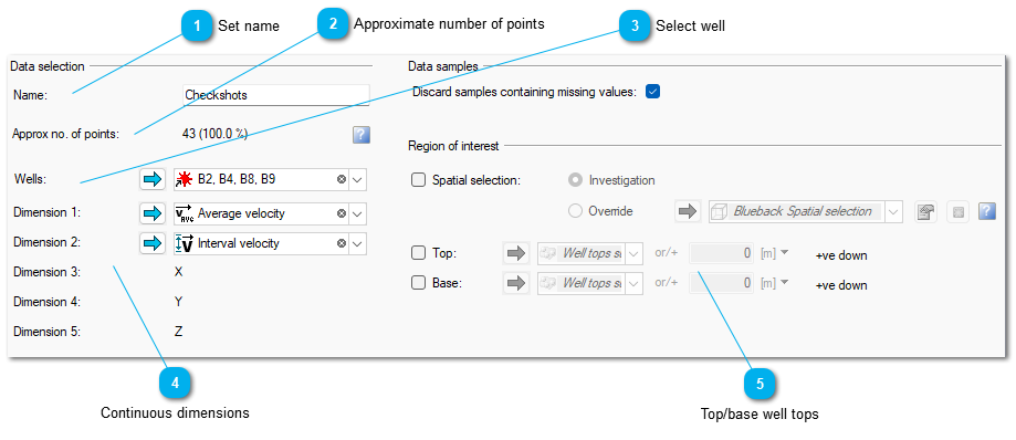 {width="6.197916666666667in" height="2.6770833333333335in"}]
[
{width="0.4166666666666667in" height="0.4166666666666667in"}]{.underline}[Set name]{.underline}[
 {width="3.5833333333333335in" height="0.2916666666666667in"}]
[Text field where the dataset name can be specified.]
[
{width="0.4166666666666667in" height="0.4166666666666667in"}]{.underline}[Approximate number of points]{.underline}[
 {width="3.5625in" height="0.25in"}]
[Shows the number of points that the selected data contains. The percentage shown is how many percent of the available points that contribute to the investigation.]
[
{width="0.4166666666666667in" height="0.4166666666666667in"}]{.underline}[Select well]{.underline}[
 {width="3.5104166666666665in" height="0.375in"}]
[Select the wells to be included in the investigation.]
[
{width="0.4166666666666667in" height="0.4166666666666667in"}]{.underline}[Continuous dimensions]{.underline}[
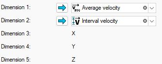 {width="3.4791666666666665in" height="1.375in"}]
[Select the individual continuous checkshot attributes. If a template for an axis has not already been selected, then it will be set the first time data is selected.]
[
{width="0.4166666666666667in" height="0.4166666666666667in"}]{.underline}[Top/base well tops]{.underline}[
 {width="4.520833333333333in" height="0.7083333333333334in"}]
[If your project has well tops you can filter the number of points. A offset to the well tops can also be added. If no well top is selected you can specify a value to constrain your investigation against. The two options can also be combined:]
[
 {width="3.4375in" height="0.6458333333333334in"}]
[All region of interest values refer to TVD values. (Not Measured Depth.)]
[Model]{.underline}
[Allows model properties for a selected grid to be selected.]
[
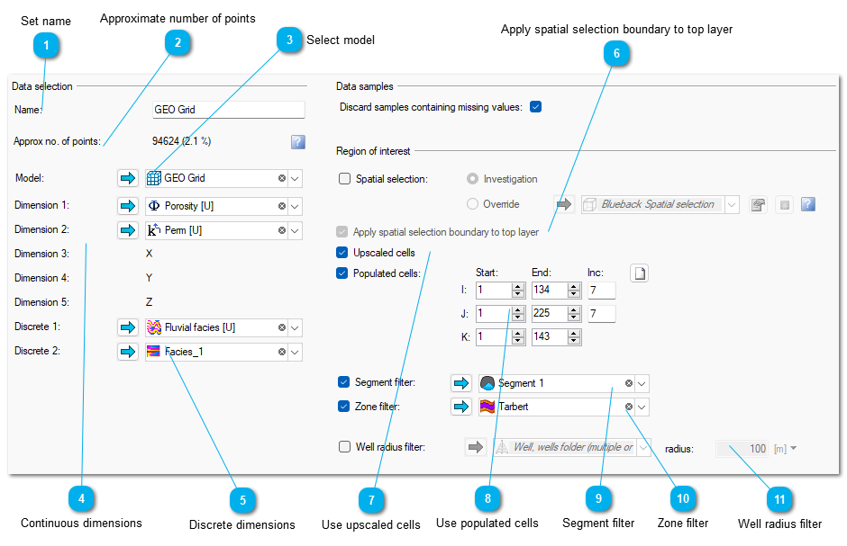 {width="6.197916666666667in" height="4.0in"}]
[If segment or zone filter options are selected, then data can be colored and/or filtered by these selections.]
[To color by zone or segment, select the appropriate option from the ]{.underline}[color data by]{.underline}[ option.]
[
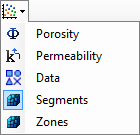 {width="1.4583333333333333in" height="1.40625in"} ]
[To filter the data, select the required segments or zones from the data points drop down menu icon.]
[
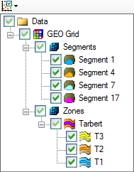 {width="1.96875in" height="2.5208333333333335in"}]
[Additionally, model property data can be filtered to only show points within a given radius of selected wells. Again, the selected wells can be filtered in the data points drop down menu icon.]
[
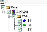 {width="1.96875in" height="1.3541666666666667in"}]
[
{width="0.4166666666666667in" height="0.4166666666666667in"}]{.underline}[Set name]{.underline}[
 {width="3.5104166666666665in" height="0.2916666666666667in"}]
[Text field where the dataset name can be specified.]
[
{width="0.4166666666666667in" height="0.4166666666666667in"}]{.underline}[Approximate number of points]{.underline}[
 {width="3.5in" height="0.28125in"}]
[Shows the number of points that the selected data contains. The percentage shown is how many percent of the available points that contribute to the investigation.]
[
{width="0.4166666666666667in" height="0.4166666666666667in"}]{.underline}[Select model]{.underline}[
 {width="3.4895833333333335in" height="0.3125in"}]
[Select a model grid. The other controls will be populated with data from the selected grid.]
[
{width="0.4166666666666667in" height="0.4166666666666667in"}]{.underline}[Continuous dimensions]{.underline}[
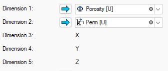 {width="3.5in" height="1.4895833333333333in"}]
[Select the model properties for each continuous dimension. If a template for a dimension has not already been selected, then it will be set the first time data is selected.]
[
{width="0.4166666666666667in" height="0.4166666666666667in"}]{.underline}[Discrete dimensions]{.underline}[
 {width="3.5in" height="0.6875in"}]
[Select the model properties for each discrete dimension. If a template for a dimension has not already been selected, then it will be set the first time data is selected.]
[
{width="0.4166666666666667in" height="0.4166666666666667in"}]{.underline}[Apply spatial selection boundary to top layer]{.underline}[
 {width="2.5625in" height="0.28125in"}]
[Filter the selected data according to cells within one or more selected polygons]
[The boundary filter can be applied to the X & Y coordinates of the top layer, and all the cells in those pillars plotted (below left - selected points in green), or the X & Y coordinate of each individual cell can be considered, so for non-vertical grids, the selected cells may belong to different columns at different depths (below right).]
[
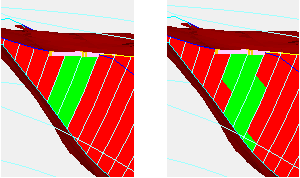 {width="3.125in" height="1.8541666666666667in"}]
[
{width="0.4166666666666667in" height="0.4166666666666667in"}]{.underline}[Use upscaled cells]{.underline}[
 {width="1.2604166666666667in" height="0.3333333333333333in"}]
[This includes the upscaled cells in the property. ]
[
{width="0.4166666666666667in" height="0.4166666666666667in"}]{.underline}[Use populated cells]{.underline}[
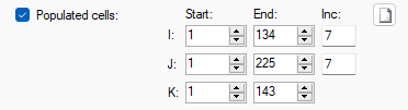 {width="3.875in" height="1.0520833333333333in"}]
[Includes the populated (E.g. property modelled properties) cells into the investigation. ]
[This control allow a subsection of the propagated data to be plotted, and/or the data decimated. When data is first selected, the decimation will be set so that there are less than 100,000 points selected. The decimation can be altered as required or the "reset" button can be used to ensure no decimation is applied. ]
[Note that the value of 100,000 is somewhat arbitrary - the performance of the plot will depend on your hardware configuration.]
[
{width="0.4166666666666667in" height="0.4166666666666667in"}]{.underline}[Segment filter]{.underline}[
 {width="3.78125in" height="0.28125in"}]
[Filter the selected data according to model segments]
[
{width="0.4166666666666667in" height="0.4166666666666667in"}]{.underline}[Zone filter]{.underline}[
 {width="3.7708333333333335in" height="0.2708333333333333in"}]
[Filter the selected data according to model zones]
[
{width="0.4166666666666667in" height="0.4166666666666667in"}]{.underline}[Well radius filter]{.underline}[
 {width="5.291666666666667in" height="0.28125in"}]
[Filter the selected data according to cells within a given radius of one or more selected wells ]
[Point sets]{.underline}
[Allows pointsets and their properties to be selected.]
[
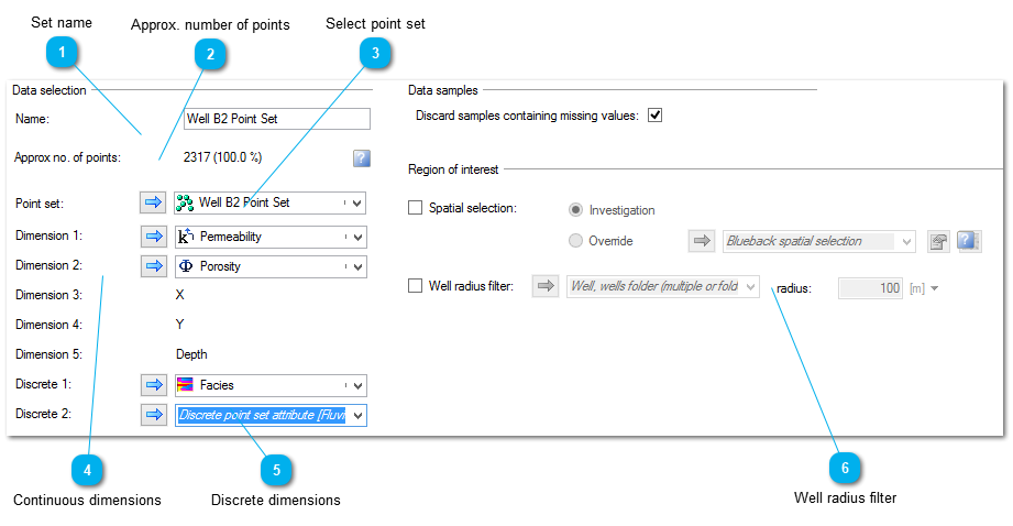 {width="6.197916666666667in" height="3.2083333333333335in"}]
[
{width="0.4166666666666667in" height="0.4166666666666667in"}]{.underline}[Set name]{.underline}[
 {width="3.4895833333333335in" height="0.3020833333333333in"}]
[Text field where the dataset name can be specified.]
[
{width="0.4166666666666667in" height="0.4166666666666667in"}]{.underline}[Approx. number of points]{.underline}[
 {width="3.5520833333333335in" height="0.2916666666666667in"}]
[Shows the number of points that the selected data contains. The percentage shown is how many percent of the available points that contribute to the investigation.]
[
{width="0.4166666666666667in" height="0.4166666666666667in"}]{.underline}[Select point set]{.underline}[
 {width="3.4375in" height="0.28125in"}]
[Select the point set to be plotted]
[
{width="0.4166666666666667in" height="0.4166666666666667in"}]{.underline}[Continuous dimensions]{.underline}[
 {width="3.4479166666666665in" height="1.3958333333333333in"}]
[Select the point set properties for each continuous dimension. If a template for a dimension has not already been selected, then it will be set the first time data is selected.]
[
{width="0.4166666666666667in" height="0.4166666666666667in"}]{.underline}[Discrete dimensions]{.underline}[
 {width="3.5104166666666665in" height="0.6041666666666666in"}]
[Select the point set properties for each discrete dimension. If a template for a dimension has not already been selected, then it will be set the first time data is selected.]
[
{width="0.4166666666666667in" height="0.4166666666666667in"}]{.underline}[Well radius filter]{.underline}[
 {width="5.166666666666667in" height="0.2708333333333333in"}]
[Filter the selected data according to cells within a given radius of one or more selected wells ]
[Realization folders]{.underline}
[Allows properties from a group of realization folders to be selected. These properties can be considered as a single dataset or as child datasets (one per realization folder) much like well logs are currently supported.]
[
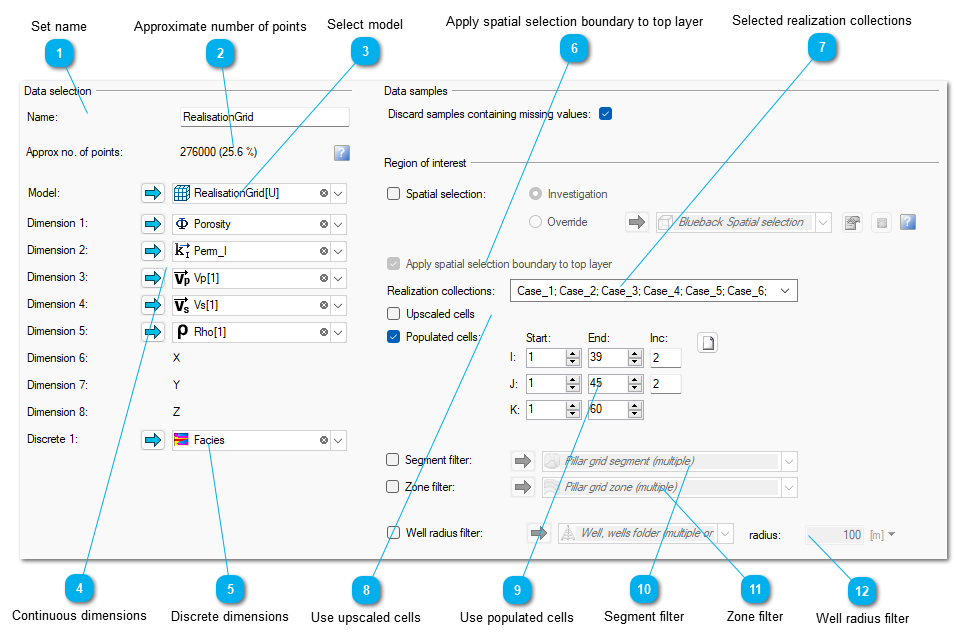 {width="6.197916666666667in" height="4.15625in"}]
[Each child realization folder will be identifiable within the investigation and data can have its color/appearance etc controlled.]
[If segment or zone filter options are selected, then data can be colored and/or filtered by these selections.]
[To color by zone or segment, select the appropriate option from the color data by option.]
[
{width="1.4583333333333333in" height="1.40625in"} ][To filter the data, select the required segments or zones from the data points drop down menu icon.]
[
{width="1.96875in" height="2.5208333333333335in"}][Additionally, model property data can be filtered to only show points within a given radius of selected wells. Again, the selected wells can be filtered in the data points drop down menu icon.]
[
{width="1.96875in" height="1.3541666666666667in"}][
{width="0.4166666666666667in" height="0.4166666666666667in"}]{.underline}[Set name]{.underline}[
 {width="3.5104166666666665in" height="0.2916666666666667in"}]
[Text field where the dataset name can be specified.]
[
{width="0.4166666666666667in" height="0.4166666666666667in"}]{.underline}[Approximate number of points]{.underline}[
 {width="3.5in" height="0.28125in"}]
[Shows the number of points that the selected data contains. The percentage shown is how many percent of the available points that contribute to the investigation.]
[
{width="0.4166666666666667in" height="0.4166666666666667in"}]{.underline}[Select model]{.underline}[
 {width="3.4895833333333335in" height="0.3125in"}]
[Select a model grid. The other controls will be populated with data from the selected grid.]
[
{width="0.4166666666666667in" height="0.4166666666666667in"}]{.underline}[Continuous dimensions]{.underline}[
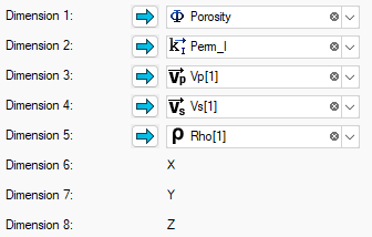 {width="3.5in" height="2.2291666666666665in"}]
[Select the model properties for each continuous dimension. If a template for a dimension has not already been selected, then it will be set the first time data is selected.]
[
{width="0.4166666666666667in" height="0.4166666666666667in"}]{.underline}[Discrete dimensions]{.underline}[
 {width="3.5in" height="0.3645833333333333in"}]
[Select the model properties for each discrete dimension. If a template for a dimension has not already been selected, then it will be set the first time data is selected.]
[
{width="0.4166666666666667in" height="0.4166666666666667in"}]{.underline}[Apply spatial selection boundary to top layer]{.underline}[
 {width="4.5in" height="0.28125in"}]
[Filter the selected data according to cells within one or more selected polygons]
[The boundary filter can be applied to the X & Y coordinates of the top layer, and all the cells in those pillars plotted (below left - selected points in green), or the X & Y coordinate of each individual cell can be considered, so for non-vertical grids, the selected cells may belong to different columns at different depths (below right).]
[
{width="3.125in" height="1.8541666666666667in"}][
{width="0.4166666666666667in" height="0.4166666666666667in"}]{.underline}[Selected realization collections]{.underline}[
 {width="4.447916666666667in" height="0.2916666666666667in"}]
[This allows the user to select the realization collections to be included in the dataset. ]
[If the selected dimension property is defined within a realization collection then all selected collections must also contain a property with the same name. ]
[
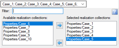 {width="4.135416666666667in" height="1.6875in"}]
[
{width="0.4166666666666667in" height="0.4166666666666667in"}]{.underline}[Use upscaled cells]{.underline}[
 {width="1.1666666666666667in" height="0.2708333333333333in"}]
[This includes the upscaled cells in the property. ]
[
{width="0.4166666666666667in" height="0.4166666666666667in"}]{.underline}[Use populated cells]{.underline}[
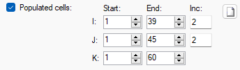 {width="3.5833333333333335in" height="1.0520833333333333in"}]
[Includes the populated (E.g. property modelled properties) cells into the investigation. ]
[This control allow a subsection of the propagated data to be plotted, and/or the data decimated. When data is first selected, the decimation will be set so that there are less than 100,000 points selected. The decimation can be altered as required or the "reset" button can be used to ensure no decimation is applied. ]
[Note that the value of 100,000 is somewhat arbitrary - the performance of the plot will depend on your hardware configuration.]
[
{width="0.4166666666666667in" height="0.4166666666666667in"}]{.underline}[Segment filter]{.underline}[
 {width="4.520833333333333in" height="0.28125in"}]
[Filter the selected data according to model segments]
[
{width="0.4166666666666667in" height="0.4166666666666667in"}]{.underline}[Zone filter]{.underline}[
 {width="4.5in" height="0.2708333333333333in"}]
[Filter the selected data according to model zones]
[
{width="0.4166666666666667in" height="0.4166666666666667in"}]{.underline}[Well radius filter]{.underline}[
 {width="5.447916666666667in" height="0.28125in"}]
[Filter the selected data according to cells within a given radius of one or more selected wells ]
[Seismic 2D]{.underline}
[Allows 2D seismic lines to be selected. All selected lines must have the same geometry.]
[
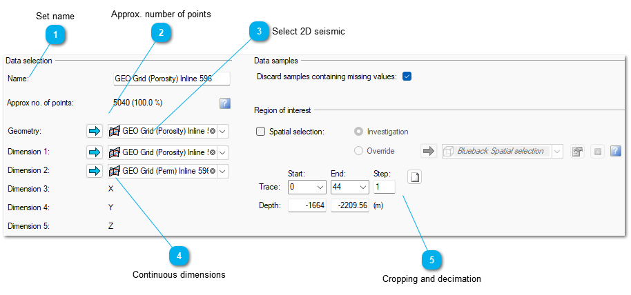 {width="6.197916666666667in" height="2.8958333333333335in"}]
[
{width="0.4166666666666667in" height="0.4166666666666667in"}]{.underline}[Set name]{.underline}[
 {width="3.4791666666666665in" height="0.3125in"}]
[Text field where the dataset name can be specified.]
[
{width="0.4166666666666667in" height="0.4166666666666667in"}]{.underline}[Approx. number of points]{.underline}[
 {width="3.4270833333333335in" height="0.3229166666666667in"}]
[Shows the number of points that the selected data contains. The percentage shown is how many percent of the available points that contribute to the investigation.]
[
{width="0.4166666666666667in" height="0.4166666666666667in"}]{.underline}[Select 2D seismic]{.underline}[
 {width="3.4791666666666665in" height="0.3125in"}]
[Select the 2D seismic geometry.]
[
{width="0.4166666666666667in" height="0.4166666666666667in"}]{.underline}[Continuous dimensions]{.underline}[
 {width="3.5104166666666665in" height="1.4270833333333333in"}]
[Select the seismic 2D properties for each continuous dimension. If a template for a dimension has not already been selected, then it will be set the first time data is selected.]
[
{width="0.4166666666666667in" height="0.4166666666666667in"}]{.underline}[Cropping and decimation]{.underline}[
 {width="2.65625in" height="0.8645833333333334in"}]
[This control allow a subsection of the propagated data to be plotted, and/or the data decimated. When data is first selected, the decimation will be set so that there are less than 100,000 points selected. The decimation can be altered as required or the "reset" button can be used to ensure no decimation is applied. ]
[Note that the value of 100,000 is somewhat arbitrary - the performance of the plot will depend on your hardware configuration.]
[Seismic 2D by vintage]{.underline}
[Projects often contain many 2D lines. By taking advantage of Petrel's seismic 'vintage' functionality this option allows multiple 2D seismic "intage properties"to selected in one go and treated as one item. The vintage can be used in a manner similar to global well logs for well data, but with the exception that the seismic vintage is not physically tied to a template.]
[First, create a vintage for each template e.g. a porosity vintage, a permeability vintage, etc. Then, for each 2D survey, assign the unique geometry lines to each vintage. Finally, by selecting the vintages in the dimension area the seismic 2D lines belonging to that vintage will be selected and included in the investigation.]
[As the vintages may contain 2D lines of different lengths, it is not possible to limit the data by line number. However the line increment and the z-range can be set to limit the data.]
[There are some limitations:]
[A 2D seismic survey can only contain 1 unique 2D line geometry for each vintage.]
[Each vintage can only contain data belonging to the same domain - a mixture of domains between or across vintages is not allowed.]
[Lines from different vintages will be matched by their survey geometry. Any unmatched lines will be ignored.]
[The number of 2D lines belonging to each vintage must be the same.]
[
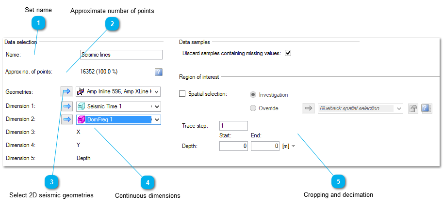 {width="6.197916666666667in" height="2.8958333333333335in"}]
[
{width="0.4166666666666667in" height="0.4166666666666667in"}]{.underline}[Set name]{.underline}[
 {width="3.5104166666666665in" height="0.28125in"}]
[Text field where the dataset name can be specified.]
[
{width="0.4166666666666667in" height="0.4166666666666667in"}]{.underline}[Approximate number of points]{.underline}[
 {width="3.46875in" height="0.28125in"}]
[Shows the number of points that the selected data contains. The percentage shown is how many percent of the available points that contribute to the investigation.]
[
{width="0.4166666666666667in" height="0.4166666666666667in"}]{.underline}[Select 2D seismic geometries]{.underline}[
 {width="3.4583333333333335in" height="0.3125in"}]
[Select the 2D lines to be used as geometries in the investigation dataset. Only unique lines will be selected.]
[
{width="0.4166666666666667in" height="0.4166666666666667in"}]{.underline}[Continuous dimensions]{.underline}[
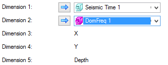 {width="3.53125in" height="1.375in"}]
[Select the seismic 2D properties for each continuous dimension. If a template for a dimension has not already been selected, then it will be set the first time data is selected.]
[
{width="0.4166666666666667in" height="0.4166666666666667in"}]{.underline}[Cropping and decimation]{.underline}[
 {width="2.4791666666666665in" height="0.7708333333333334in"}]
[These controls allow the data to be decimated by trace, and/or a vertical subsection of the selected data to be plotted.]
[Seismic 3D]{.underline}
[Allows 3D seismic cubes to be selected. All selected seismic cubes must have the same geometry.]
[
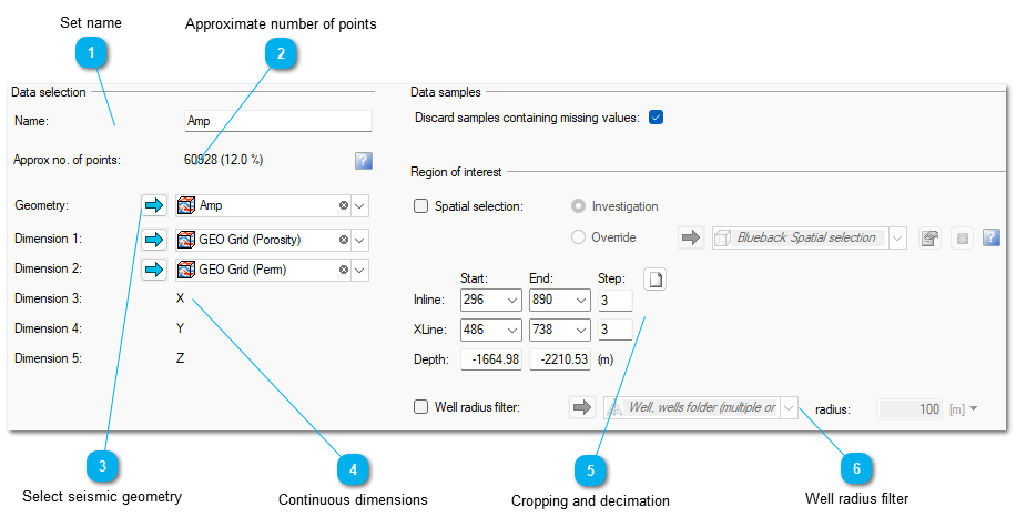 {width="6.197916666666667in" height="3.2083333333333335in"}]
[
{width="0.4166666666666667in" height="0.4166666666666667in"}]{.underline}[Set name]{.underline}[
 {width="3.4270833333333335in" height="0.3229166666666667in"}]
[Text field where the dataset name can be specified.]
[
{width="0.4166666666666667in" height="0.4166666666666667in"}]{.underline}[Approximate number of points]{.underline}[
 {width="3.4895833333333335in" height="0.3020833333333333in"}]
[Shows the number of points that the selected data contains. The percentage shown is how many percent of the available points that contribute to the investigation.]
[
{width="0.4166666666666667in" height="0.4166666666666667in"}]{.underline}[Select seismic geometry]{.underline}[
 {width="3.4791666666666665in" height="0.3229166666666667in"}]
[Select the seismic 3D cube to be used as the geometry template. All properties added to the dataset needs to conform to the seismic geometry set in this field.]
[
{width="0.4166666666666667in" height="0.4166666666666667in"}]{.underline}[Continuous dimensions]{.underline}[
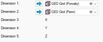 {width="3.5416666666666665in" height="1.4375in"}]
[Select the seismic 3D properties for each continuous dimension. If a template for a dimension has not already been selected, then it will be set the first time data is selected.]
[
{width="0.4166666666666667in" height="0.4166666666666667in"}]{.underline}[Cropping and decimation]{.underline}[
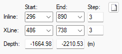 {width="2.5104166666666665in" height="1.1145833333333333in"}]
[This control allow a subsection of the propagated data to be plotted, and/or the data decimated. When data is first selected, the decimation will be set so that there are less than 100,000 points selected. The decimation can be altered as required or the "reset" button can be used to ensure no decimation is applied. ]
[Note that the value of 100,000 is somewhat arbitrary - the performance of the plot will depend on your hardware configuration.]
[
{width="0.4166666666666667in" height="0.4166666666666667in"}]{.underline}[Well radius filter]{.underline}[
 {width="5.4375in" height="0.3125in"}]
[Filter the selected data according to cells within a given radius of one or more selected wells ]
[Simulation cases]{.underline}
[Allows properties from a group of simulation cases to be selected. These properties can be considered as a single dataset or as child datasets (one per simulation case) much like well logs are currently supported.]
[
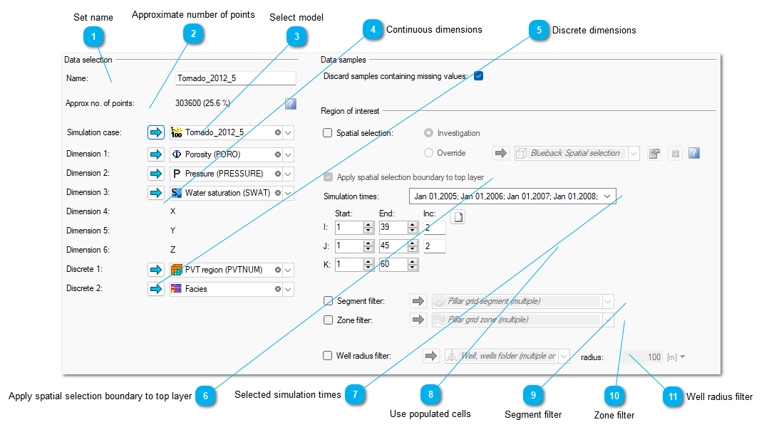 {width="6.197916666666667in" height="3.5in"}]
[Each child timestep will be identifiable within the investigation and data can have its color/appearance etc controlled.]
[If segment or zone filter options are selected, then data can be colored and/or filtered by these selections.]
[To color by zone or segment, select the appropriate option from the color data by option.]
[
{width="1.4583333333333333in" height="1.40625in"} ][To filter the data, select the required segments or zones from the data points drop down menu icon.]
[
{width="1.96875in" height="2.5208333333333335in"}][Additionally, model property data can be filtered to only show points within a given radius of selected wells. Again, the selected wells can be filtered in the data points drop down menu icon.]
[
{width="1.96875in" height="1.3541666666666667in"}][
{width="0.4166666666666667in" height="0.4166666666666667in"}]{.underline}[Set name]{.underline}[
 {width="3.5104166666666665in" height="0.2916666666666667in"}]
[Text field where the dataset name can be specified.]
[
{width="0.4166666666666667in" height="0.4166666666666667in"}]{.underline}[Approximate number of points]{.underline}[
 {width="3.5in" height="0.28125in"}]
[Shows the number of points that the selected data contains. The percentage shown is how many percent of the available points that contribute to the investigation.]
[
{width="0.4166666666666667in" height="0.4166666666666667in"}]{.underline}[Select model]{.underline}[
 {width="3.4895833333333335in" height="0.3125in"}]
[Select a model grid. The other controls will be populated with data from the selected grid.]
[
{width="0.4166666666666667in" height="0.4166666666666667in"}]{.underline}[Continuous dimensions]{.underline}[
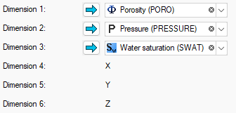 {width="3.5in" height="1.6770833333333333in"}]
[Select the model properties for each continuous dimension. If a template for a dimension has not already been selected, then it will be set the first time data is selected.]
[
{width="0.4166666666666667in" height="0.4166666666666667in"}]{.underline}[Discrete dimensions]{.underline}[
 {width="3.5in" height="0.6354166666666666in"}]
[Select the model properties for each discrete dimension. If a template for a dimension has not already been selected, then it will be set the first time data is selected.]
[
{width="0.4166666666666667in" height="0.4166666666666667in"}]{.underline}[Apply spatial selection boundary to top layer]{.underline}[
 {width="4.5in" height="0.28125in"}]
[Filter the selected data according to cells within one or more selected polygons]
[The boundary filter can be applied to the X & Y coordinates of the top layer, and all the cells in those pillars plotted (below left - selected points in green), or the X & Y coordinate of each individual cell can be considered, so for non-vertical grids, the selected cells may belong to different columns at different depths (below right).]
[
{width="3.125in" height="1.8541666666666667in"}][
{width="0.4166666666666667in" height="0.4166666666666667in"}]{.underline}[Selected simulation times]{.underline}[
 {width="4.447916666666667in" height="0.2916666666666667in"}]
[This allows the user to select the simulation timesteps to be included in the dataset. ]
[
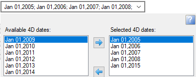 {width="4.104166666666667in" height="1.6145833333333333in"}]
[
{width="0.4166666666666667in" height="0.4166666666666667in"}]{.underline}[Use populated cells]{.underline}[
 {width="3.4791666666666665in" height="1.0520833333333333in"}]
[Includes the populated (E.g. property modelled properties) cells into the investigation. ]
[This control allow a subsection of the propagated data to be plotted, and/or the data decimated. When data is first selected, the decimation will be set so that there are less than 100,000 points selected. The decimation can be altered as required or the "reset" button can be used to ensure no decimation is applied. ]
[Note that the value of 100,000 is somewhat arbitrary - the performance of the plot will depend on your hardware configuration.]
[
{width="0.4166666666666667in" height="0.4166666666666667in"}]{.underline}[Segment filter]{.underline}[
 {width="4.520833333333333in" height="0.28125in"}]
[Filter the selected data according to model segments]
[
{width="0.4166666666666667in" height="0.4166666666666667in"}]{.underline}[Zone filter]{.underline}[
 {width="4.5in" height="0.2708333333333333in"}]
[Filter the selected data according to model zones]
[
{width="0.4166666666666667in" height="0.4166666666666667in"}]{.underline}[Well radius filter]{.underline}[
 {width="5.447916666666667in" height="0.28125in"}]
[Filter the selected data according to cells within a given radius of one or more selected wells ]
[Summary results]{.underline}
[Allows properties from a group of summary results to be selected. These properties can be considered as a single dataset or as child datasets (one per summary result) much like well logs are currently supported.]
[Bt default, summary results will be displayed as a statistical fan in time series plots. Display of the fan and each individual summary result can be controlled by the user as necessary. ]
[
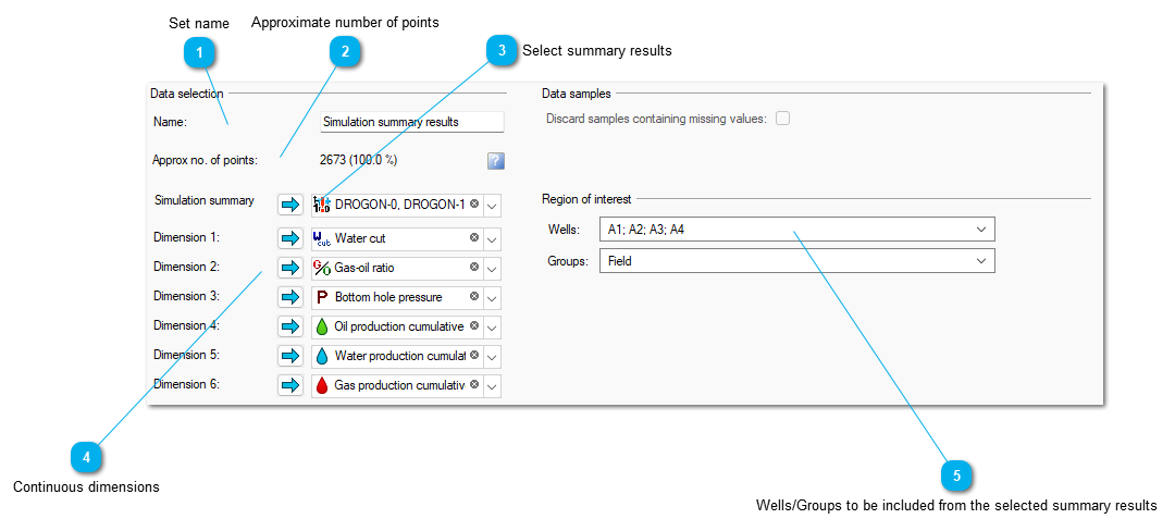 {width="6.197916666666667in" height="2.7916666666666665in"}]
[
{width="0.4166666666666667in" height="0.4166666666666667in"}]{.underline}[Set name]{.underline}[
 {width="3.5833333333333335in" height="0.2916666666666667in"}]
[Text field where the dataset name can be specified.]
[
{width="0.4166666666666667in" height="0.4166666666666667in"}]{.underline}[Approximate number of points]{.underline}[
 {width="3.5625in" height="0.25in"}]
[Shows the number of points that the selected data contains. The percentage shown is how many percent of the available points that contribute to the investigation.]
[
{width="0.4166666666666667in" height="0.4166666666666667in"}]{.underline}[Select summary results]{.underline}[
 {width="3.5104166666666665in" height="0.375in"}]
[Select the summary results to be included in this dataset.]
[
{width="0.4166666666666667in" height="0.4166666666666667in"}]{.underline}[Continuous dimensions]{.underline}[
 {width="3.4791666666666665in" height="1.75in"}]
[Select the continuous observed data properties. If a template for an axis has not already been selected, then it will be set the first time data is selected.]
[
{width="0.4166666666666667in" height="0.4166666666666667in"}]{.underline}[Wells/Groups to be included from the selected summary results]{.underline}[
 {width="4.989583333333333in" height="0.6354166666666666in"}]
[Summary results can contain 1 or more wells and optional groups These controls can be used to select a subset of wells and/or groups to be included.]
[Surface]{.underline}
[Allows properties for a selected surface to be selected.]
[
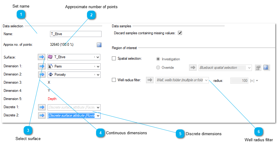 {width="6.197916666666667in" height="3.2708333333333335in"}]
[
{width="0.4166666666666667in" height="0.4166666666666667in"}]{.underline}[Set name]{.underline}[
 {width="3.5416666666666665in" height="0.3125in"}]
[Text field where the dataset name can be specified.]
[
{width="0.4166666666666667in" height="0.4166666666666667in"}]{.underline}[Approximate number of points]{.underline}[
 {width="3.5729166666666665in" height="0.3229166666666667in"}]
[Shows the number of points that the selected data contains. The percentage shown is how many percent of the available points that contribute to the investigation.]
[
{width="0.4166666666666667in" height="0.4166666666666667in"}]{.underline}[Select surface]{.underline}[
 {width="3.40625in" height="0.3229166666666667in"}]
[Select surface to be included as a dataset in the investigation.]
[
{width="0.4166666666666667in" height="0.4166666666666667in"}]{.underline}[Continuous dimensions]{.underline}[
 {width="3.4479166666666665in" height="1.40625in"}]
[Select the surface properties for each continuous dimension. If a template for a dimension has not already been selected, then it will be set the first time data is selected.]
[
{width="0.4166666666666667in" height="0.4166666666666667in"}]{.underline}[Discrete dimensions]{.underline}[
 {width="3.5104166666666665in" height="0.6458333333333334in"}]
[Select the surface properties for each discrete dimension. If a template for a dimension has not already been selected, then it will be set the first time data is selected.]
[
{width="0.4166666666666667in" height="0.4166666666666667in"}]{.underline}[Well radius filter]{.underline}[
 {width="5.145833333333333in" height="0.3229166666666667in"}]
[Filter the selected data according to cells within a given radius of one or more selected wells ]
[Table data]{.underline}
[Allows table data to be selected. This could be pasted from excel or loaded via a csv file.]
[
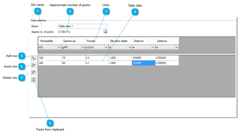 {width="6.197916666666667in" height="3.5in"}]
[
{width="0.4166666666666667in" height="0.4166666666666667in"}]{.underline}[Set name]{.underline}[
 {width="3.5729166666666665in" height="0.3020833333333333in"}]
[Set a name for the table data]
[
{width="0.4166666666666667in" height="0.4166666666666667in"}]{.underline}[Approximate number of points]{.underline}[
 {width="3.59375in" height="0.2708333333333333in"}]
[Shows the number of points that the selected data contains. The percentage shown is how many percent of the available points that contribute to the investigation.]
[
{width="0.4166666666666667in" height="0.4166666666666667in"}]{.underline}[Units]{.underline}[
 {width="6.197916666666667in" height="0.6145833333333334in"}]
[Allows the units of the column to be selected. They are linked to the defined dimensions.]
[
{width="0.4166666666666667in" height="0.4166666666666667in"}]{.underline}[Table data]{.underline}[
 {width="6.197916666666667in" height="0.5520833333333334in"}]
[Editable table with point data.]
[The table can contain cells that or blank or NaN. How these cells are processed depends on the discard samples containing missing values option.]
[
{width="0.4166666666666667in" height="0.4166666666666667in"}]{.underline}[Add row]{.underline}[
 {width="0.3645833333333333in" height="0.3645833333333333in"}]
[A new row is added to the bottom of the table]
[
{width="0.4166666666666667in" height="0.4166666666666667in"}]{.underline}[Insert row]{.underline}[
 {width="0.3645833333333333in" height="0.3645833333333333in"}]
[A new row is inserted above the currently selected row]
[
{width="0.4166666666666667in" height="0.4166666666666667in"}]{.underline}[Delete row]{.underline}[
 {width="0.3645833333333333in" height="0.3645833333333333in"}]
[The currently selected row is deleted]
[
{width="0.4166666666666667in" height="0.4166666666666667in"}]{.underline}[Paste from clipboard]{.underline}[
 {width="0.3645833333333333in" height="0.3645833333333333in"}]
[There are two subtly different ways to paste data into the table from the clipboard:]
[Using this button effectively deletes the current table and replaces it with data from the clipboard. All information in the current table is lost, even if the new table has smaller dimensions than the old one.]
[Using the right-click menu option in each individual table cell. ]
[This will insert the data from the clipboard below and to the right of the selected cell, i.e. the selected cell is replaced with the first cell from the clipboard. ]
[If more rows are required than are present on inserting the data then these will be added. ]
[However, the same is not true for columns. The number of columns is controlled by the number of templates selected. Therefore the inserted table is truncated horizontally as required. This option is particularly useful for combining datasets.]
[Volumetric cases]{.underline}
[Allows a group of volume results to be selected. These volume results can be considered as a single dataset or as child datasets (one per volume result) much like well logs are currently supported.]
[Volumetric datasets are different to all other datasets as follows:]
[It is not possible to combine volumetric datasets and other datatypes in the same investigation.]
[It is not possible to use region of interest or spatial selections with volumetric cases.]
[Only volumetric results can be selected as continuous dimensions. All possible results can be selected irrespective of the results chosen during the volume calculation. If a selected volume result not available then the dimension will not contain any values.]
[Discrete dimensions will be automatically determined from the volume calculation options.]
[Note: Loading volumetric case data via Ocean is slow. Creating a volumetric dataset will display a warning informing the user of this and asking if they want to proceed.]{.underline}
[
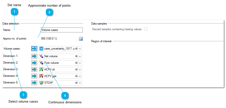 {width="6.197916666666667in" height="2.96875in"}]
[
{width="0.4166666666666667in" height="0.4166666666666667in"}]{.underline}[Set name]{.underline}[
 {width="3.5104166666666665in" height="0.2916666666666667in"}]
[Text field where the dataset name can be specified.]
[
{width="0.4166666666666667in" height="0.4166666666666667in"}]{.underline}[Approximate number of points]{.underline}[
 {width="3.5in" height="0.28125in"}]
[Shows the number of points that the selected data contains. The percentage shown is how many percent of the available points that contribute to the investigation.]
[
{width="0.4166666666666667in" height="0.4166666666666667in"}]{.underline}[Select volume cases]{.underline}[
 {width="3.4895833333333335in" height="0.3125in"}]
[Select the volume cases.]
[
{width="0.4166666666666667in" height="0.4166666666666667in"}]{.underline}[Continuous dimensions]{.underline}[
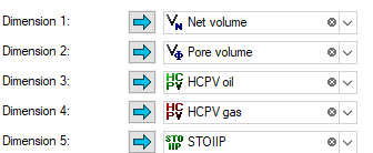 {width="3.5in" height="1.4375in"}]
[Select the volume calculation result properties for each continuous dimension.]
[Well logs]{.underline}
[Allows well logs for the selected wells to be selected.]
[
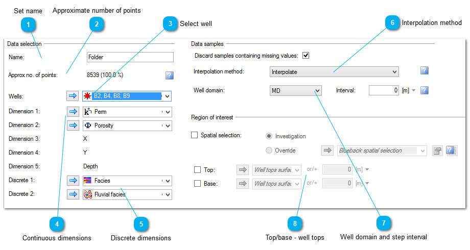 {width="6.197916666666667in" height="3.2916666666666665in"}]
[
{width="0.4166666666666667in" height="0.4166666666666667in"}]{.underline}[Set name]{.underline}[
 {width="3.5833333333333335in" height="0.2916666666666667in"}]
[Text field where the dataset name can be specified.]
[
{width="0.4166666666666667in" height="0.4166666666666667in"}]{.underline}[Approximate number of points]{.underline}[
 {width="3.5625in" height="0.25in"}]
[Shows the number of points that the selected data contains. The percentage shown is how many percent of the available points that contribute to the investigation.]
[
{width="0.4166666666666667in" height="0.4166666666666667in"}]{.underline}[Select well]{.underline}[
 {width="3.5104166666666665in" height="0.375in"}]
[Select the wells to be included in the investigation.]
[
{width="0.4166666666666667in" height="0.4166666666666667in"}]{.underline}[Continuous dimensions]{.underline}[
 {width="3.4791666666666665in" height="1.4166666666666667in"}]
[Select the continuous global well logs. If a template for an axis has not already been selected, then it will be set the first time data is selected.]
[
{width="0.4166666666666667in" height="0.4166666666666667in"}]{.underline}[Discrete dimensions]{.underline}[
 {width="3.4895833333333335in" height="0.6354166666666666in"}]
[Select the discrete global well logs from the selected well. If a template for an axis has not already been selected, then it will be set the first time data is selected.]
[
{width="0.4166666666666667in" height="0.4166666666666667in"}]{.underline}[Interpolation method]{.underline}[
 {width="4.979166666666667in" height="0.2916666666666667in"}]
[The allows the user to control how Blueback Investigator handles well logs that have different sampling intervals.]
[The interpolation options are described here]{.underline}.
[
{width="0.4166666666666667in" height="0.4166666666666667in"}]{.underline}[Well domain and step interval]{.underline}[
 {width="4.989583333333333in" height="0.2916666666666667in"}]
[If the interpolation method is Interpolate then the user can use these controls to set domain in which interpolation occurs and the sampling interval that should be applied.]
[The user can select from MD, TVD and TWT domains.]
[The default values are MD with an interval of 0. This means Blueback Investigator will sample the logs in MD using the most common MD step found from the selected logs.]
[These controls allow the user to select any sampling interval and the domain required. For example, when comparing well log data to seismic data, it might be useful to choose the domain and interval to match that of the seismic data.]
[
{width="0.4166666666666667in" height="0.4166666666666667in"}]{.underline}[Top/base - well tops]{.underline}[
 {width="3.8125in" height="0.6145833333333334in"}]
[If your project has well tops you can filter the number of points. A offset to the well tops can also be added. If no well top is selected you can specify a value to constrain your investigation against. The two options can also be combined:]
[
{width="3.4375in" height="0.6458333333333334in"}][All region of interest values refer to TVD values. (Not Measured Depth.)]
[Well observed data]{.underline}
[Allows observed data for the selected observed dataset to be selected.]
[
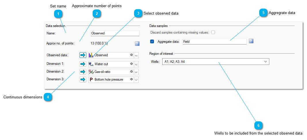 {width="6.197916666666667in" height="2.8333333333333335in"}]
[
{width="0.4166666666666667in" height="0.4166666666666667in"}]{.underline}[Set name]{.underline}[
 {width="3.5833333333333335in" height="0.2916666666666667in"}]
[Text field where the dataset name can be specified.]
[
{width="0.4166666666666667in" height="0.4166666666666667in"}]{.underline}[Approximate number of points]{.underline}[
 {width="3.5625in" height="0.25in"}]
[Shows the number of points that the selected data contains. The percentage shown is how many percent of the available points that contribute to the investigation.]
[
{width="0.4166666666666667in" height="0.4166666666666667in"}]{.underline}[Select observed data]{.underline}[
 {width="3.5104166666666665in" height="0.375in"}]
[Select the observed data to be included in the investigation.]
[
{width="0.4166666666666667in" height="0.4166666666666667in"}]{.underline}[Continuous dimensions]{.underline}[
 {width="3.4791666666666665in" height="1.0in"}]
[Select the continuous observed data properties. If a template for an axis has not already been selected, then it will be set the first time data is selected.]
[
{width="0.4166666666666667in" height="0.4166666666666667in"}]{.underline}[Aggregrate data]{.underline}[
 {width="4.979166666666667in" height="0.3645833333333333in"}]
[This allows the user to create a new identifier that aggregate of the data from the selected wells.]
[
{width="0.4166666666666667in" height="0.4166666666666667in"}]{.underline}[Wells to be included from the selected observed data]{.underline}[
 {width="4.989583333333333in" height="0.2916666666666667in"}]
[Observed data can contain 1 or more wells. This control can be used to select a subset of wells to be included if that is required. ]
[Well points]{.underline}
[Allows well point logs for the selected wells to be selected.]
[
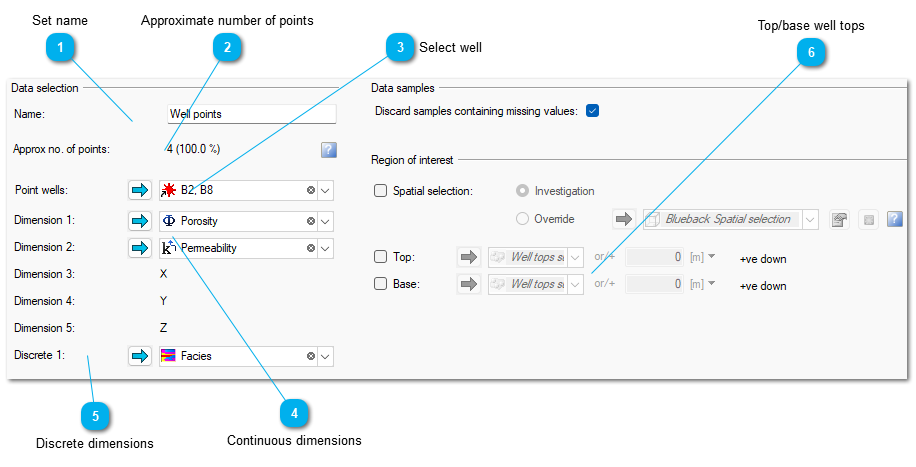 {width="6.197916666666667in" height="3.15625in"}]
[
{width="0.4166666666666667in" height="0.4166666666666667in"}]{.underline}[Set name]{.underline}[
 {width="3.5833333333333335in" height="0.2916666666666667in"}]
[Text field where the dataset name can be specified.]
[
{width="0.4166666666666667in" height="0.4166666666666667in"}]{.underline}[Approximate number of points]{.underline}[
 {width="3.5625in" height="0.25in"}]
[Shows the number of points that the selected data contains. The percentage shown is how many percent of the available points that contribute to the investigation.]
[
{width="0.4166666666666667in" height="0.4166666666666667in"}]{.underline}[Select well]{.underline}[
 {width="3.5104166666666665in" height="0.375in"}]
[Select the wells to be included in the investigation.]
[
{width="0.4166666666666667in" height="0.4166666666666667in"}]{.underline}[Continuous dimensions]{.underline}[
 {width="3.4791666666666665in" height="1.375in"}]
[Select the individual continuous well point data. If a template for an axis has not already been selected, then it will be set the first time data is selected.]
[
{width="0.4166666666666667in" height="0.4166666666666667in"}]{.underline}[Discrete dimensions]{.underline}[
 {width="3.4895833333333335in" height="0.2916666666666667in"}]
[Select the individual discrete well point data. If a template for an axis has not already been selected, then it will be set the first time data is selected.]
[
{width="0.4166666666666667in" height="0.4166666666666667in"}]{.underline}[Top/base well tops]{.underline}[
 {width="4.385416666666667in" height="0.5833333333333334in"}]
[If your project has well tops you can filter the number of points. A offset to the well tops can also be added. If no well top is selected you can specify a value to constrain your investigation against. The two options can also be combined:]
[
{width="3.4375in" height="0.6458333333333334in"}][All region of interest values refer to TVD values. (Not Measured Depth.)]
[Well tops]{.underline}
[Allows well top properties for the selected wells to be selected.]
[
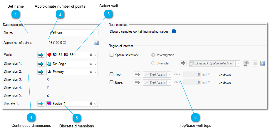 {width="6.197916666666667in" height="3.0416666666666665in"}]
[
{width="0.4166666666666667in" height="0.4166666666666667in"}]{.underline}[Set name]{.underline}[
 {width="3.5833333333333335in" height="0.2916666666666667in"}]
[Text field where the dataset name can be specified.]
[
{width="0.4166666666666667in" height="0.4166666666666667in"}]{.underline}[Approximate number of points]{.underline}[
 {width="3.5625in" height="0.25in"}]
[Shows the number of points that the selected data contains. The percentage shown is how many percent of the available points that contribute to the investigation.]
[
{width="0.4166666666666667in" height="0.4166666666666667in"}]{.underline}[Select well]{.underline}[
 {width="3.5104166666666665in" height="0.375in"}]
[Select the wells to be included in the investigation.]
[
{width="0.4166666666666667in" height="0.4166666666666667in"}]{.underline}[Continuous dimensions]{.underline}[
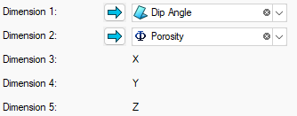 {width="3.4791666666666665in" height="1.3645833333333333in"}]
[Select the individual continuous well top attributes. If a template for an axis has not already been selected, then it will be set the first time data is selected.]
[
{width="0.4166666666666667in" height="0.4166666666666667in"}]{.underline}[Discrete dimensions]{.underline}[
 {width="3.4895833333333335in" height="0.2916666666666667in"}]
[Select the individual discrete well top attributes. If a template for an axis has not already been selected, then it will be set the first time data is selected.]
[
{width="0.4166666666666667in" height="0.4166666666666667in"}]{.underline}[Top/base well tops]{.underline}[
 {width="4.4375in" height="0.625in"}]
[If your project has well tops you can filter the number of points. A offset to the well tops can also be added. If no well top is selected you can specify a value to constrain your investigation against. The two options can also be combined:]
[
{width="3.4375in" height="0.6458333333333334in"}][All region of interest values refer to TVD values. (Not Measured Depth.)]
[Dimensions]{.underline}
[The dimension definition can be edited by selected the required column header.]
[
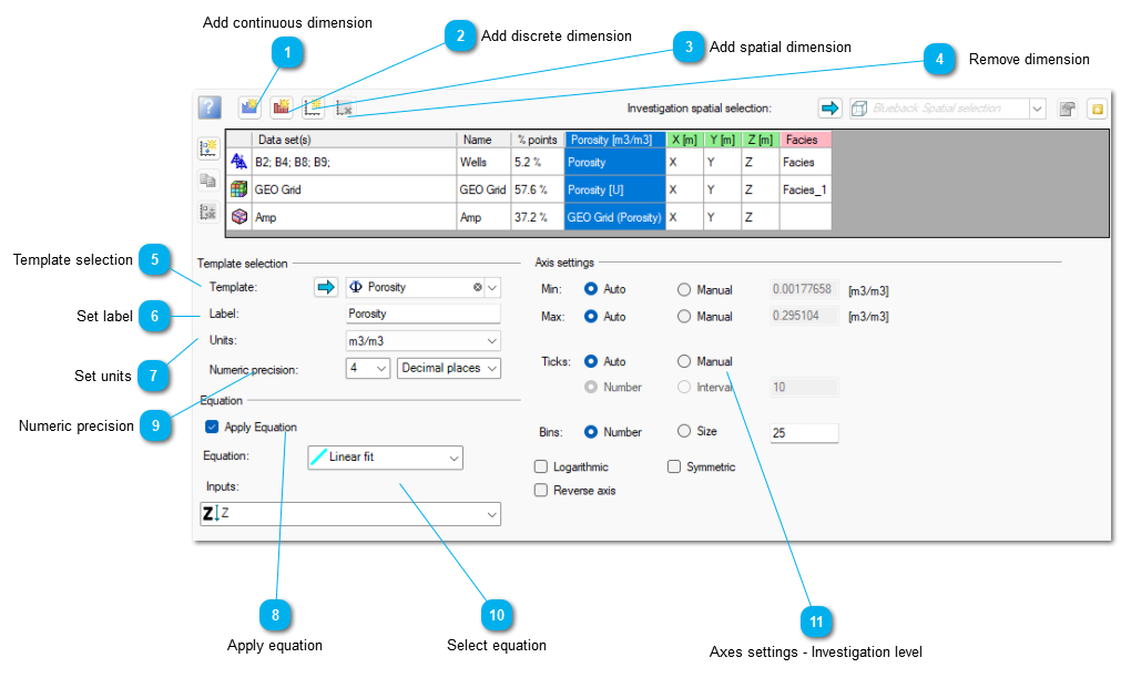 {width="6.197916666666667in" height="3.75in"}]
[
{width="0.4166666666666667in" height="0.4166666666666667in"}]{.underline}[Add continuous dimension]{.underline}[
 {width="0.3229166666666667in" height="0.3645833333333333in"}]
[Adds a new continuous dimension into the investigation.]
[
{width="0.4166666666666667in" height="0.4166666666666667in"}]{.underline}[Add discrete dimension]{.underline}[
 {width="0.34375in" height="0.3645833333333333in"}]
[Adds a new discrete dimension into the investigation.]
[
{width="0.4166666666666667in" height="0.4166666666666667in"}]{.underline}[Add spatial dimension]{.underline}[
 {width="0.3125in" height="0.3645833333333333in"}]
[Adds a new spatial dimension into the investigation.]
[
{width="0.4166666666666667in" height="0.4166666666666667in"}]{.underline}[ Remove dimension]{.underline}[
 {width="0.34375in" height="0.3645833333333333in"}]
[Delete the highlighted column in the table.]
[
{width="0.4166666666666667in" height="0.4166666666666667in"}]{.underline}[Template selection]{.underline}[
 {width="3.1354166666666665in" height="0.3333333333333333in"}]
[Controls the selected template for the dimension]
[
{width="0.4166666666666667in" height="0.4166666666666667in"}]{.underline}[Set label]{.underline}[
 {width="3.1666666666666665in" height="0.28125in"}]
[Set display name of the dimension. The label name will be used in all the plots. Default is to have the same label name as the Template name.]
[
{width="0.4166666666666667in" height="0.4166666666666667in"}]{.underline}[Set units]{.underline}[
 {width="3.2083333333333335in" height="0.3333333333333333in"}]
[Set the display units for the dimension.]
[
{width="0.4166666666666667in" height="0.4166666666666667in"}]{.underline}[Apply equation]{.underline}[
 {width="1.1041666666666667in" height="0.2916666666666667in"}]
[Controls whether an equation should be used when dimension is missing data.]
[
{width="0.4166666666666667in" height="0.4166666666666667in"}]{.underline}[Numeric precision]{.underline}[
 {width="3.1354166666666665in" height="0.2916666666666667in"}]
[Set the numeric precision to which data from this dimension should be displayed. ]
[Precision can be expressed as either:]
[number of decimal places]
[number of significant figures]
[engineering precision]
[
{width="0.4166666666666667in" height="0.4166666666666667in"}]{.underline}[Select equation]{.underline}[
 {width="3.1145833333333335in" height="0.9166666666666666in"}]
[Controls which equation should be used for this calculated dimension. After selecting an equation it is necessary to select the inputs as required.]
[
{width="0.4166666666666667in" height="0.4166666666666667in"}]{.underline}[Axes settings - Investigation level]{.underline}[
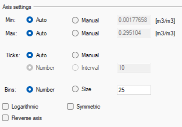 {width="3.7916666666666665in" height="2.65625in"}]
[Controls the Investigation level axes settings for windows. See Axis settings]{.underline} for more information
[Import table data]{.underline}
[Text data files can be imported directly into a defined investigation. ]
[Example]{.underline}
[Investigation with 3 Dimensions:]
[
 {width="1.6979166666666667in" height="1.3958333333333333in"}]
[Right-click on the ]{.underline}[investigation]{.underline}[ and select ]{.underline}[Import table data]{.underline}[:]
[
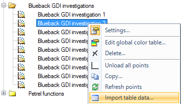 {width="3.84375in" height="2.21875in"}]
[Select text file in dialog and update ]{.underline}[Delimiter]{.underline}[ and ]{.underline}[Number of header lines]{.underline}[ fields to match the input data. Press ]{.underline}[Import]{.underline}[:]
[
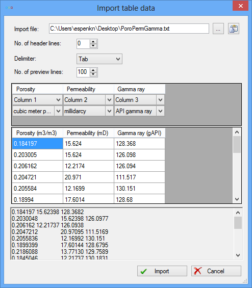 {width="5.145833333333333in" height="5.885416666666667in"}]
[Open investigation. A new table dataset has been added to the investigation:]
[
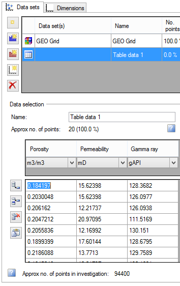 {width="3.6875in" height="5.854166666666667in"}]
[Data loading report]{.underline}
[The data loading report provides information about number of valid/invalid samples in each dataset and the reason why a sample was discarded.]
[If necessary the investigation will be loaded before showing the report. ]
[
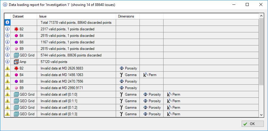 {width="6.197916666666667in" height="3.0208333333333335in"}]
[Windows]{.underline}
[The basic functionality for each of the Blueback Investigator plots is driven from the toolbars in the window. There are three types of window:]
[Histogram window]{.underline} - for creating histograms and viewing statistics
[Crossplot window]{.underline} - a 2D scatterplot, but with optional horizontal and vertical histograms attached, displaying the horizontal axis and vertical axis data respectively.
[Matrix window]{.underline} - plot multiple dimensions at once in a matrix
[Parallel coordinates window]{.underline} - quickly identify trends in the investigation data
[Blueback Investigator 3D plot]{.underline} - plot dimensions in 3D space
[Petrel 3D window]{.underline} - visualize spatial investigations in the Petrel 3D window
[General]{.underline}
[The following sections apply to the majority of Blueback Investigator windows:]
[Window control panel]{.underline}
[The window control panel aims to improve usability by making it mush easier for the user to control what is visible in the window. ]
[The control panel can be hidden using this
 {width="0.3125in" height="0.23958333333333334in"} and shown using this
  {width="0.23958333333333334in" height="0.25in"} toolbar button.]
[
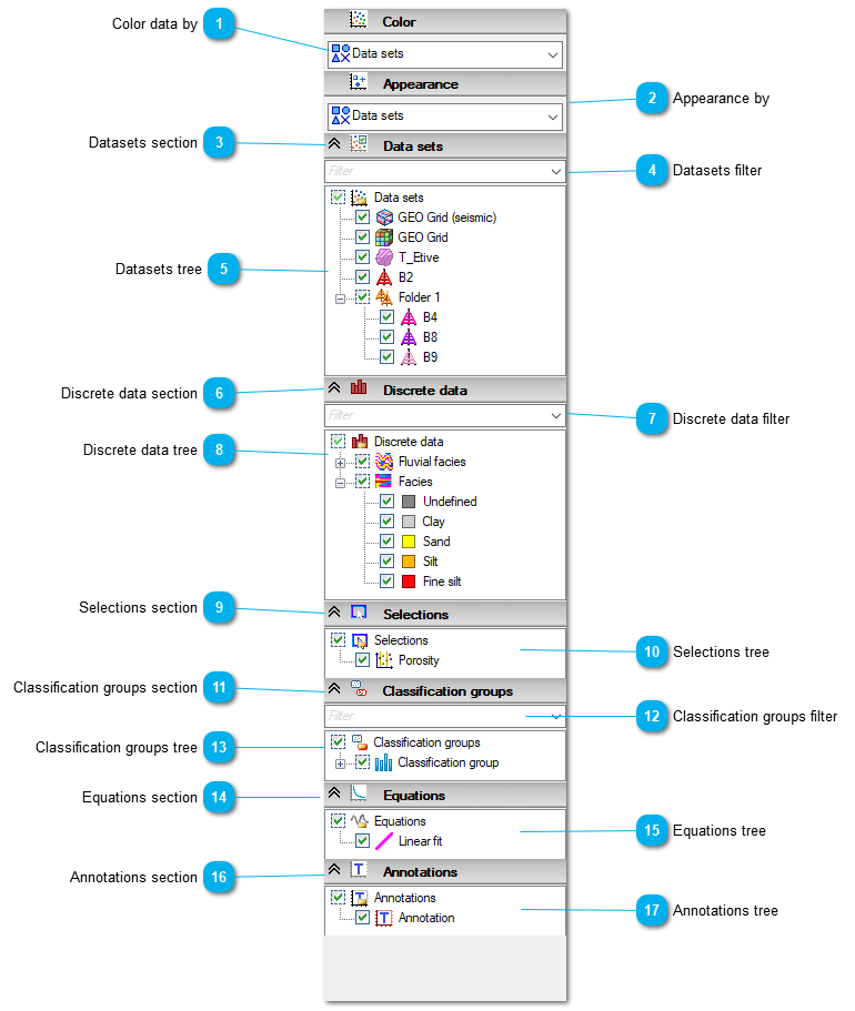 {width="6.197916666666667in" height="7.322916666666667in"}]
[
{width="0.4166666666666667in" height="0.4166666666666667in"}]{.underline}[Color data by]{.underline}[
 {width="2.21875in" height="0.5833333333333334in"}]
[Use this to select how the data should be colored (see Coloring of data]{.underline})
[
{width="0.4166666666666667in" height="0.4166666666666667in"}]{.underline}[Appearance by]{.underline}[
 {width="2.2604166666666665in" height="0.59375in"}]
[Use this to select the appearance to the points to be used (see Appearance of data]{.underline})
[
{width="0.4166666666666667in" height="0.4166666666666667in"}]{.underline}[Datasets section]{.underline}[
 {width="1.8020833333333333in" height="0.25in"}]
[This section marks the top of the dataset controls. The section can be collapsed/expanded by double clicking on this header.]
[
{width="0.4166666666666667in" height="0.4166666666666667in"}]{.underline}[Datasets filter]{.underline}[
 {width="2.3125in" height="0.2916666666666667in"}]
[The content in the datasets tree will be filter to those names that contain the filter string.]
[Note: When the filter is applied, toggling on/off the tree will only affect the shown datasets rather than all the datasets.]{.underline}
[
{width="0.4166666666666667in" height="0.4166666666666667in"}]{.underline}[Datasets tree]{.underline}[
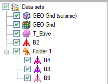 {width="2.2604166666666665in" height="1.7708333333333333in"}]
[Toggle items in the tree to change the visibility of data from the datasets. The dataset context menu will be displayed via the right mouse button.]
[
{width="0.4166666666666667in" height="0.4166666666666667in"}]{.underline}[Discrete data section]{.underline}[
 {width="1.8541666666666667in" height="0.2604166666666667in"}]
[This section marks the top of the discrete data controls. The section can be collapsed/expanded by double clicking on this header.]
[
{width="0.4166666666666667in" height="0.4166666666666667in"}]{.underline}[Discrete data filter]{.underline}[
 {width="2.2916666666666665in" height="0.25in"}]
[The content in the discrete data tree will be filter to those names that contain the filter string.]
[Note: When the filter is applied, toggling on/off the tree will only affect the shown discrete data rather than all the discrete data.]{.underline}
[
{width="0.4166666666666667in" height="0.4166666666666667in"}]{.underline}[Discrete data tree]{.underline}[
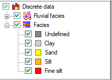 {width="2.2916666666666665in" height="1.6354166666666667in"}]
[Toggle items in the tree to change the visibility of data marked with discrete data. The discrete data context menu will be displayed via the right mouse button.]
[
{width="0.4166666666666667in" height="0.4166666666666667in"}]{.underline}[Selections section]{.underline}[
 {width="1.84375in" height="0.25in"}]
[This section marks the top of the selections controls. The section can be collapsed/expanded by double clicking on this header.]
[
{width="0.4166666666666667in" height="0.4166666666666667in"}]{.underline}[Selections tree]{.underline}[
 {width="1.8333333333333333in" height="0.46875in"}]
[Toggle items in the tree to change the selections being applied in the window.]
[
{width="0.4166666666666667in" height="0.4166666666666667in"}]{.underline}[Classification groups section]{.underline}[
 {width="1.8958333333333333in" height="0.25in"}]
[This section marks the top of the classification group controls. The section can be collapsed/expanded by double clicking on this header.]
[
{width="0.4166666666666667in" height="0.4166666666666667in"}]{.underline}[Classification groups filter]{.underline}[
 {width="2.25in" height="0.28125in"}]
[The content in the classification groups tree will be filter to those names that contain the filter string.]
[Note: When the filter is applied, toggling on/off the tree will only affect the shown classification groups rather than all the classification groups.]{.underline}
[
{width="0.4166666666666667in" height="0.4166666666666667in"}]{.underline}[Classification groups tree]{.underline}[
 {width="2.2708333333333335in" height="0.4791666666666667in"}]
[Toggle items in the tree to change the visibility of data within the classification groups. The classification groups context menu will be displayed via the right mouse button.]
[
{width="0.4166666666666667in" height="0.4166666666666667in"}]{.underline}[Equations section]{.underline}[
 {width="1.8125in" height="0.2604166666666667in"}]
[This section marks the top of the equation controls. The section can be collapsed/expanded by double clicking on this header.]
[
{width="0.4166666666666667in" height="0.4166666666666667in"}]{.underline}[Equations tree]{.underline}[
 {width="1.8333333333333333in" height="0.5in"}]
[Toggle items in the tree to change the visibility of equations in the window. The equations context menu will be displayed via the right mouse button.]
[The Distributions will appear in the Equations tree.]
[
{width="2.71875in" height="1.6666666666666667in"}][
{width="0.4166666666666667in" height="0.4166666666666667in"}]{.underline}[Annotations section]{.underline}[
 {width="2.28125in" height="0.25in"}]
[This section marks the top of the annotation controls. The section can be collapsed/expanded by double clicking on this header.]
[
{width="0.4166666666666667in" height="0.4166666666666667in"}]{.underline}[Annotations tree]{.underline}[
 {width="2.2604166666666665in" height="0.5416666666666666in"}]
[Toggle items in the tree to change the visibility of annotation in the window. The annotations context menu will be displayed via the right mouse button.]
[Dataset tree context menus]{.underline}
[Save data]{.underline}
[It is possible to save data from the Control data drop down data tree. To save data access the control data point button and right mouse click on the data you want to export. The hierarchy level in the control data tree decides what data that is exported.]
[
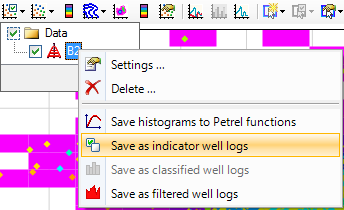 {width="3.5833333333333335in" height="2.1875in"}]
[Model data - zone and segment control]{.underline}
[Right-click on a Model in the tree displays additional visibility controls:]
[
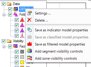 {width="3.2083333333333335in" height="2.3645833333333335in"}]
[Once displayed the controls can be removed if necessary:]
[
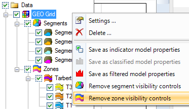 {width="3.8854166666666665in" height="2.2395833333333335in"}]
[Link visible objects]{.underline}
[It is possible to link multiple windows to the same windows control tree. This is achieved using either the toolbar button (
 {width="0.2604166666666667in" height="0.2604166666666667in"}) or the investigation context menu. ]
[Linking can be performed when the same investigation is displayed in more than 1 window. If the investigation is displayed in more than 2 windows then the user will be prompted to select the window to be linked with.]
[It is very helpful to link visible object. It allows the user to view different perspectives of the investigation in different windows at the same while ensuring that the same samples are displayed in each. Linking the windows only links the visible datasets, discrete data, selections and classifications. This allows the different windows to display using different colors, contours, annotation etc.]
[ In this example, the same investigation is displayed in each window and these have all been linked to the windows control tree. Changes to the displayed samples will update all windows.]
[
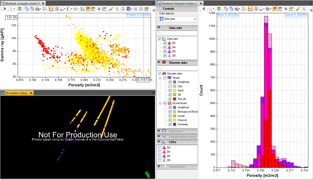 {width="6.197916666666667in" height="3.5833333333333335in"}]
[Axis settings]{.underline}
[The axis settings decides the behavior of the displayed axis in all the plots. The axis settings is tied up to the dimension templates and can be defined on the investigation level, or on a window level. ]
[View all ]{.underline}will zoom to the defined axis settings.
[Investigation level axis settings]{.underline}
[
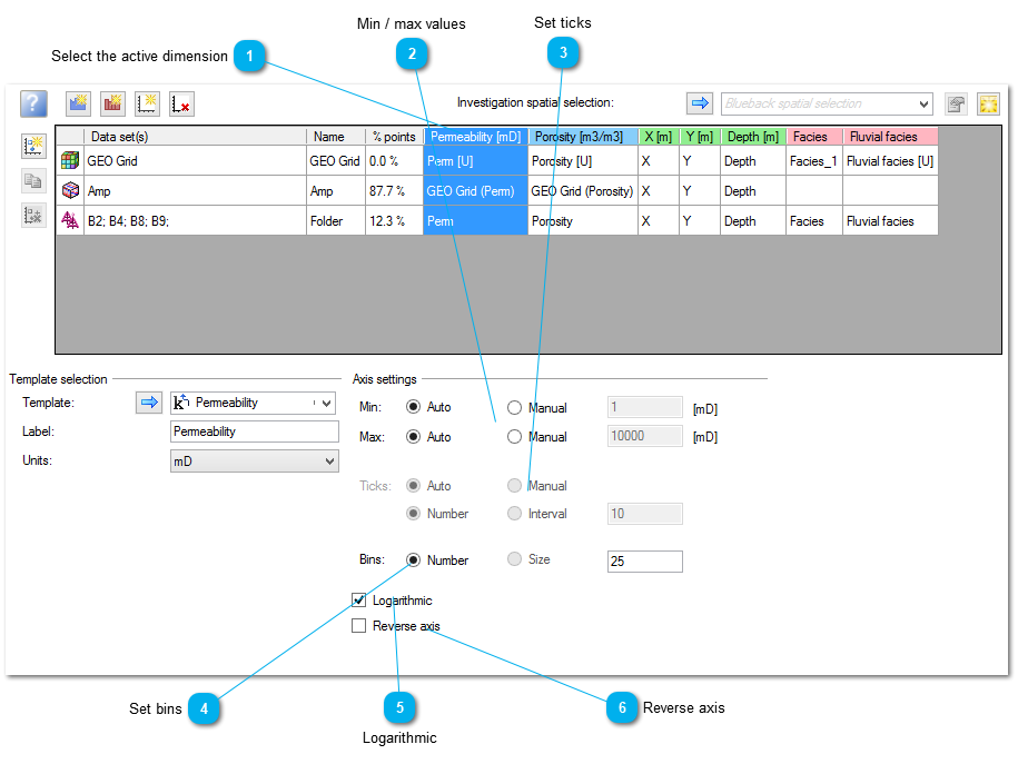 {width="6.197916666666667in" height="4.645833333333333in"}]
[
{width="0.4166666666666667in" height="0.4166666666666667in"}]{.underline}[Select the active dimension]{.underline}[
 {width="4.84375in" height="1.6458333333333333in"}]
[The selected dimension will be the active dimension.]
[
{width="0.4166666666666667in" height="0.4166666666666667in"}]{.underline}[Min / max values]{.underline}[
 {width="3.9166666666666665in" height="0.53125in"}]
[Manually set the min and max values for the dimension.]
[
{width="0.4166666666666667in" height="0.4166666666666667in"}]{.underline}[Set ticks]{.underline}[
 {width="3.2395833333333335in" height="0.5833333333333334in"}]
[Manually set the axis tick behavior. Choosing manual enables Number or Interval options.]
[
{width="0.4166666666666667in" height="0.4166666666666667in"}]{.underline}[Set bins]{.underline}[
 {width="3.21875in" height="0.2916666666666667in"}]
[Control the bin number or size]
[
{width="0.4166666666666667in" height="0.4166666666666667in"}]{.underline}[Logarithmic]{.underline}[
 {width="0.9270833333333334in" height="0.2916666666666667in"}]
[Define if the Dimension is to be treated as logarithmic in the display]
[
{width="0.4166666666666667in" height="0.4166666666666667in"}]{.underline}[Reverse axis]{.underline}[
 {width="0.9583333333333334in" height="0.2916666666666667in"}]
[Reverses the axis numbering direction.]
[Axis settings dialog]{.underline}
[
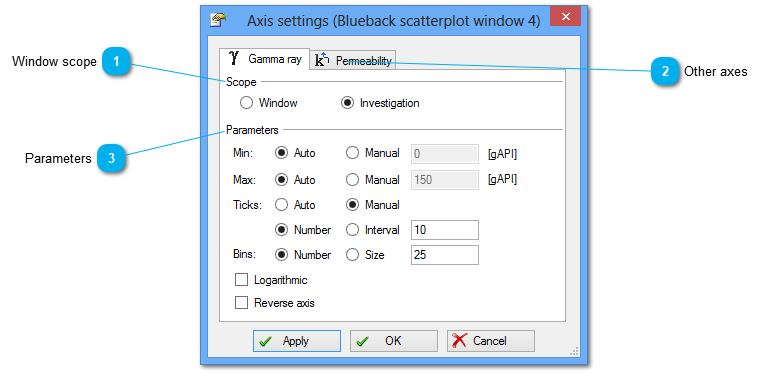 {width="6.197916666666667in" height="3.03125in"}]
[Right-click on one of the window dimension axes to display the axis settings dialog:]
[
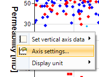 {width="2.0729166666666665in" height="1.625in"}]
[
{width="0.4166666666666667in" height="0.4166666666666667in"}]{.underline}[Window scope]{.underline}[
 {width="2.3229166666666665in" height="0.46875in"}]
[Decide scope. Investigation or Window. Changes made while in the Investigation scope will update the investigation level axis settings]{.underline}. Changes to Window will apply to the window only.
[
{width="0.4166666666666667in" height="0.4166666666666667in"}]{.underline}[Other axes]{.underline}[
 {width="1.0in" height="0.2916666666666667in"}]
[Other dimension axis settings are stored as additional tabs in the dialog.]
[
{width="0.4166666666666667in" height="0.4166666666666667in"}]{.underline}[Parameters]{.underline}[
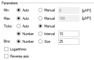 {width="3.1875in" height="2.03125in"}]
[See investigation level axis settings]{.underline} for details about the Parameters functionality.
[Legend alignment]{.underline}
[The location of both the symbol legend and colorscale can be controlled by the user. This allows the user to make better use of plot space when necessary. For example, it is often common to find one or more corners of the plots where there is no data.]
[Using the context menu it is possible to align as follows :]
[Left or right of the window ]
[In a corner inside the viewport]
[Floating - anywhere the user wants it within the window]
[For example, a legend on either side.]
[
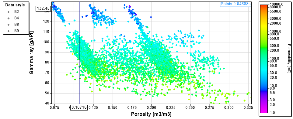 {width="6.197916666666667in" height="2.5208333333333335in"}]
[For example, legends in opposite corners]
[
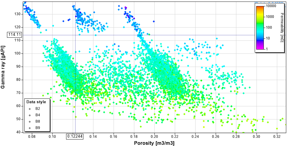 {width="6.197916666666667in" height="3.125in"}]
[Window settings]{.underline}
[The windows settings dialog]{.underline} allows the user to control the style of the window. The user choose custom colors, fonts, styles and sizes applied to the window.
[For example, the following setup is now possible:]
[
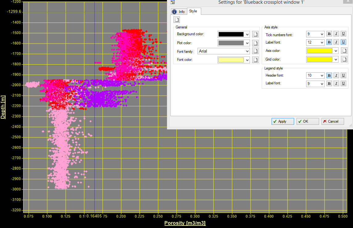 {width="6.197916666666667in" height="3.9895833333333335in"}]
[Window settings dialog]{.underline}
[The windows settings dialog allows the user to control the style of the window. The user choose custom colors, fonts, styles and sizes applied to the window. ]
[
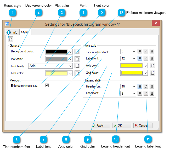 {width="6.197916666666667in" height="5.5625in"}]
[
{width="0.4166666666666667in" height="0.4166666666666667in"}]{.underline}[Reset style]{.underline}[
 {width="0.2916666666666667in" height="0.3020833333333333in"}]
[Use this to reset all window style options to the default.]
[
{width="0.4166666666666667in" height="0.4166666666666667in"}]{.underline}[Background color]{.underline}[
 {width="2.8541666666666665in" height="0.2708333333333333in"}]
[Use this to set the background color of the window.]
[
{width="0.4166666666666667in" height="0.4166666666666667in"}]{.underline}[Plot color]{.underline}[
 {width="2.84375in" height="0.28125in"}]
[Use this to set the background color of the plots in window.]
[
{width="0.4166666666666667in" height="0.4166666666666667in"}]{.underline}[Font]{.underline}[
 {width="2.8541666666666665in" height="0.2916666666666667in"}]
[Use this to set the font to be used for all text in the window. ]
[Different styles can be applied to different sections of text using other controls.]
[
{width="0.4166666666666667in" height="0.4166666666666667in"}]{.underline}[Font color]{.underline}[
 {width="2.8333333333333335in" height="0.2916666666666667in"}]
[Use this to set the color of the fonts in window.]
[
{width="0.4166666666666667in" height="0.4166666666666667in"}]{.underline}[Tick numbers font]{.underline}[
 {width="2.8229166666666665in" height="0.2916666666666667in"}]
[Use this to control the size and style of the axis tick numbers.]
[
{width="0.4166666666666667in" height="0.4166666666666667in"}]{.underline}[Label font]{.underline}[
 {width="2.8125in" height="0.2916666666666667in"}]
[Use this to control the size and style of the axis label text.]
[
{width="0.4166666666666667in" height="0.4166666666666667in"}]{.underline}[Axis color]{.underline}[
 {width="2.8125in" height="0.2916666666666667in"}]
[Use this to set the color of the axis text in plots.]
[
{width="0.4166666666666667in" height="0.4166666666666667in"}]{.underline}[Grid color]{.underline}[
 {width="2.8333333333333335in" height="0.2916666666666667in"}]
[Use this to set the color of the grid lines in plots.]
[
{width="0.4166666666666667in" height="0.4166666666666667in"}]{.underline}[Legend header font]{.underline}[
 {width="2.8020833333333335in" height="0.2916666666666667in"}]
[Use this to control the size and style of the legend header text.]
[
{width="0.4166666666666667in" height="0.4166666666666667in"}]{.underline}[Legend label font]{.underline}[
 {width="2.8229166666666665in" height="0.2916666666666667in"}]
[Use this to control the size and style of the legend text.]
[
{width="0.4166666666666667in" height="0.4166666666666667in"}]{.underline}[Enforce minimum viewport]{.underline}[
 {width="1.6458333333333333in" height="0.2916666666666667in"}]
[If checked then viewports will not be allowed to shrink smaller than a minimum size. Scroll bars will be added to the plot panel if the viewports can be drawn at the minimum size.]
[The can be particularly useful on the matrix window as it prevents viewports becoming very small.]
[Discrete plots]{.underline}
[Discrete plots and data highlighting]{.underline} allow the displayed data to be viewed in similar ways.
[Discrete plots creates a series of plots separated by the chosen discrete data (eg. Dataset, facies, zone, classification).]
[The user can select how to separate the data using the ]{.underline}[Discrete plots by]{.underline}[ (
 {width="0.28125in" height="0.22916666666666666in"}) toolbar drop-down button. Which discrete data plots are shown can be controlled by selecting the relevant entries to be visible or not in the control tree. The order of the discrete plots is controlled by the priority order of the discrete entries. The priority can be changed via the context menu or the settings dialog.]
[When discrete plots are displayed it is possible that not all viewports are visible within the window area. If this happens, it is possible that the axis labels will not be obvious for he viewports. The user can identify the plot axes for any viewport by clicking in the axis which will show a tooltip containing the axis label or my expanding the viewport (see Expanding viewports]{.underline}).
[If statistics are displayed in combination with discrete plots then the statistics will be separated by the discrete data also (see Statistics]{.underline})
[See the following for example discrete plot windows:]
[Statistics]{.underline}
[The statistics for the displayed data can be displayed in all Blueback Investigator windows. ]
[The statistics panel can be toggled using the ]{.underline}[Toggle statistics]{.underline}[ (
 {width="0.19791666666666666in" height="0.19791666666666666in"}) toolbar button.]
[The statistics are displayed in tabular form in a panel below the Blueback Investigator plots. A separate tab will be shown for each of the displayed dimensions.]
[If discrete plots are used then the statistics will be separated into the different discrete groups within each tab]
[The following image shows a Matrix plot displaying discrete plots and showing statistics:]
[
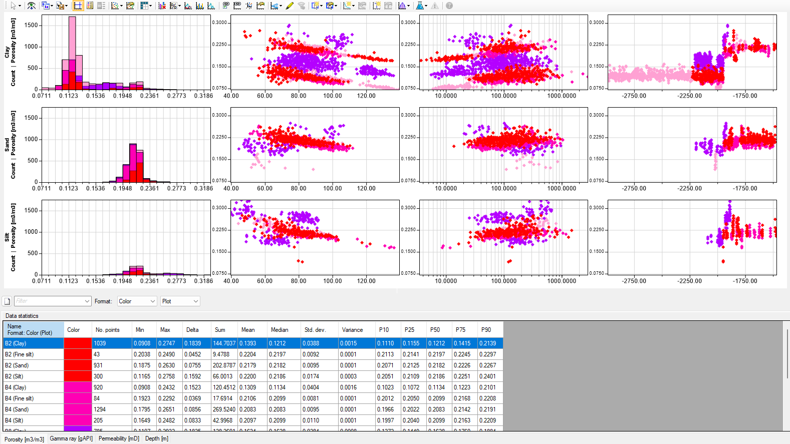 {width="6.197916666666667in" height="3.4791666666666665in"}]
[Filter/grouping controls]{.underline}
[If applicable controls are shown above the statistics table allowing the user to filter the results shown in the table and to control the format used for the Name column. ]
[The filter text field will show only entries where the name contains the given filter text. For example, the two images here show unfiltered and filter views of the same statistics:]
[
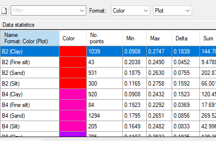 {width="4.614583333333333in" height="3.0208333333333335in"}
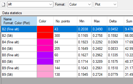 {width="4.677083333333333in" height="2.96875in"}]
[The Format controls and column sorting can be used to group the entries within the table in different ways depending on the statistics to be compared. The number of format controls shown and the options available depend on the current window setup.]
[For example, sorting the table by Name and changing the Format options can group the data either by dataset or be facies as shown in the two images here:]
[
{width="4.614583333333333in" height="3.0208333333333335in"}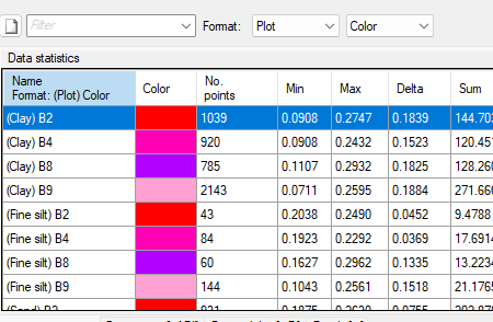 {width="4.6875in" height="3.0625in"}]
[Overlays]{.underline}
[It is possible to display simple statistics information graphically overlaid in the histogram, crossplot and matrix windows. ]
[This statistics information will be drawn as either a box plot]{.underline} (1D) or [bag plot]{.underline} (2D) graphic.
[Display of statistics overlays is controlled via the ]{.underline}[Draw statistics]{.underline}[ (
 {width="0.22916666666666666in" height="0.21875in"})option in the ]{.underline}[Statistics]{.underline}[ (
 {width="0.2604166666666667in" height="0.21875in"}) toolbar drop down menu.]
[
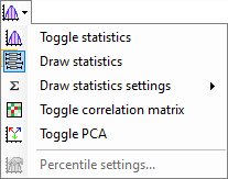 {width="2.15625in" height="1.6979166666666667in"}]
[The following image shows box and bag plots displayed over the data points in a crossplot window:]
[
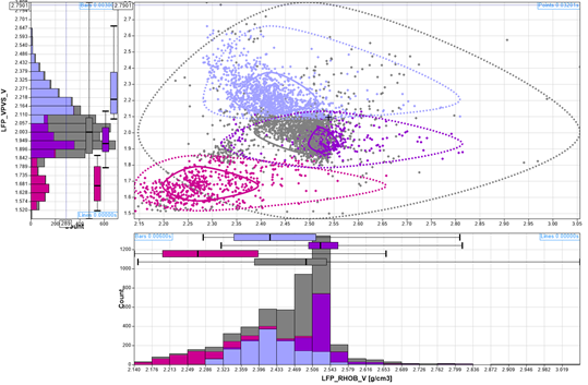 {width="5.614583333333333in" height="3.6770833333333335in"}]
[
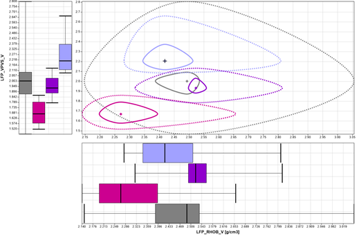 {width="5.40625in" height="3.5520833333333335in"}]
[Box plot]{.underline}
[A box plot graphically shows statistics information from a single dimension.]
[
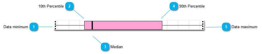 {width="6.197916666666667in" height="1.28125in"}]
[
{width="0.4166666666666667in" height="0.4166666666666667in"}]{.underline}[Data minimum]{.underline}[
 {width="0.375in" height="0.65625in"}]
[The minimum value]
[
{width="0.4166666666666667in" height="0.4166666666666667in"}]{.underline}[10th Percentile]{.underline}[
 {width="0.2916666666666667in" height="0.65625in"}]
[The value of the 10th percentile]
[
{width="0.4166666666666667in" height="0.4166666666666667in"}]{.underline}[Median]{.underline}[
 {width="0.28125in" height="0.6458333333333334in"}]
[The median value]
[
{width="0.4166666666666667in" height="0.4166666666666667in"}]{.underline}[90th Percentile]{.underline}[
 {width="0.2916666666666667in" height="0.6458333333333334in"}]
[The value of the 90th percentile]
[
{width="0.4166666666666667in" height="0.4166666666666667in"}]{.underline}[Data maximum]{.underline}[
 {width="0.2916666666666667in" height="0.625in"}]
[The maximum value]
[Bag plot]{.underline}
[A bag plot graphically shows statistics information from two dimensions. ]
[
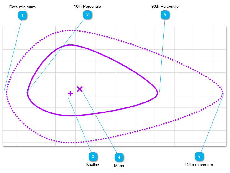 {width="6.197916666666667in" height="4.677083333333333in"}]
[The draw statistics settings menu can be used to control which features of the bag plot are rendered.]
[
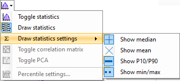 {width="3.7708333333333335in" height="1.7083333333333333in"}]
[
{width="0.4166666666666667in" height="0.4166666666666667in"}]{.underline}[Data minimum]{.underline}[
 {width="0.375in" height="0.65625in"}]
[The dashed line connects the minimum and maximum data values of the two dimensions]
[
{width="0.4166666666666667in" height="0.4166666666666667in"}]{.underline}[10th Percentile]{.underline}[
 {width="0.2916666666666667in" height="0.65625in"}]
[The solid line connects the 10th percentile and 90th percentile values of the two dimensions]
[
{width="0.4166666666666667in" height="0.4166666666666667in"}]{.underline}[Median]{.underline}[
 {width="0.28125in" height="0.6458333333333334in"}]
[The median value of the two dimensions]
[
{width="0.4166666666666667in" height="0.4166666666666667in"}]{.underline}[Mean]{.underline}[
 {width="0.2916666666666667in" height="0.2916666666666667in"}]
[The mean value of the two dimensions]
[
{width="0.4166666666666667in" height="0.4166666666666667in"}]{.underline}[90th Percentile]{.underline}[
 {width="0.2916666666666667in" height="0.6458333333333334in"}]
[The value of the 90th percentile]
[
{width="0.4166666666666667in" height="0.4166666666666667in"}]{.underline}[Data maximum]{.underline}[
 {width="0.2916666666666667in" height="0.625in"}]
[The dashed line connects the minimum and maximum data values of the two dimensions]
[Principal Component Analysis]{.underline}
[It is possible to perform Principal Component Analysis (PCA) on the displayed data in all Blueback Investigator windows excluding the histogram window.]
[Principal Component Analysis will be performed for each group of displayed data. The PCA will be performed using all the displayed displayed dimensions. For example, if colored by a discrete dimension then separate PCAs will be performed on each set of displayed discrete data.]
[The results of the PCA will be shown in a tab in the panel at the bottom of the window. The tab will contain a table showing variance and a table showing the eigenvalues.]
[To perform PCA on the data the ]{.underline}[Toggle PCA ]{.underline}[(
 {width="0.15625in" height="0.17708333333333334in"}) option should be selected from the ]{.underline}[Show data]{.underline}[ (
 {width="0.2916666666666667in" height="0.23958333333333334in"}) toolbar drop down menu.]
[
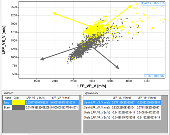 {width="5.822916666666667in" height="4.625in"}]
[Percentile-Percentile plots]{.underline}
[Percentile-Percentile plots (P-P plots) display the normal score statistical distributions of the data rather than the actual data. P-P plots are available in bother the crossplot and matrix windows.]
[P-P plots can be useful for determining how correlated different dimensions are. ]
[The plot is normal score and has a locked aspect ratio therefore the majority of toolbar options are disabled when viewing these plots. A reference line is drawn the plot at 45 degrees intersecting 0, 0.]
[To display the Percentile-Percentile plot of the data the ]{.underline}[Draw P-P plot ]{.underline}[(
 {width="0.19791666666666666in" height="0.19791666666666666in"}) option should be selected from the ]{.underline}[Show data]{.underline}[ ({width="0.2916666666666667in" height="0.23958333333333334in"}) toolbar drop down menu.]
[
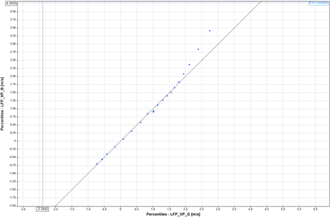 {width="5.041666666666667in" height="3.3020833333333335in"}]
[The following image shows P-P plots being used with discrete plots.]
[
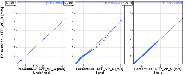 {width="6.197916666666667in" height="2.5in"}]
[Histogram]{.underline}
[The histogram window allows analysis of data matching a given template. The histogram provides 1D view through the selected data. The data is displayed as a series of bars/lines across a number of bins with the height of each bar/line representing the amount of data in each bin. The data can be displayed as either counts or percentages. ]
[The user can apply selections to the data be analyzed. Statistics can also be shown in the panel beneath the plot for the displayed data.]
[The user also has the option to annotate the plot as necessary to add notes.]
[Note: ]{.underline}
[Often the number of points on the histogram do not match the approx. no of points shown in the data selection. ]
[The reason why there is a difference between the approx. no of points and the actual number of points being displayed in the histogram is normally due to:]
[the approx no of points is indicating the total number possible points which can be plotted. For example, all the cells in a grid.]
[the actual number of points is determined by what is actually loaded. For example, any cells with no volume are discarded.]
[
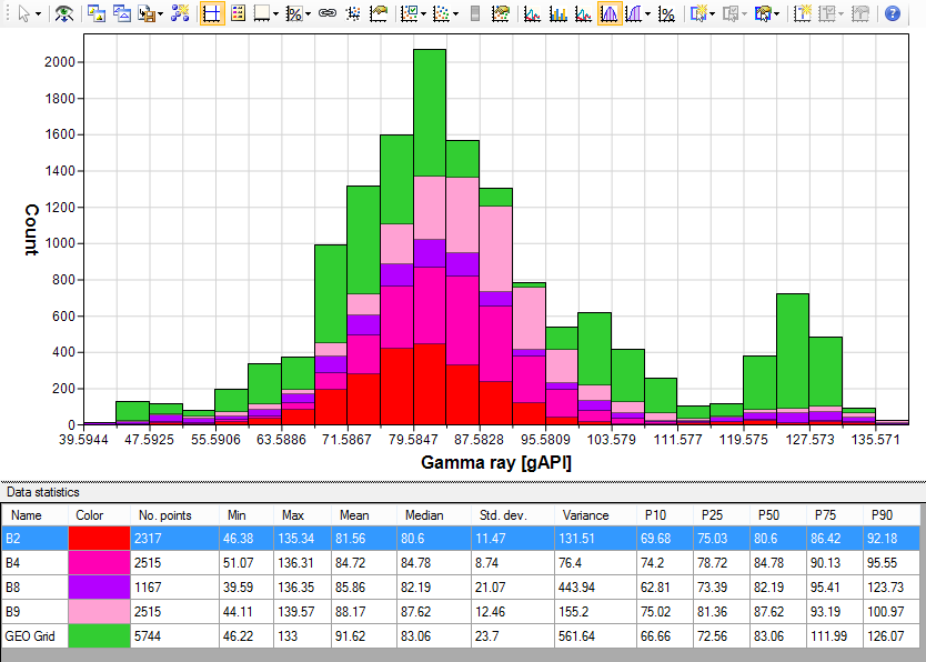 {width="6.197916666666667in" height="4.427083333333333in"}]
[Note: Data must be displayed as point data (not point density data) in order to be displayed on a histogram.]{.underline}
[Histogram axis]{.underline}
[Histograms can be displayed against the following axes:]
[Count - a simple count of the data samples]
[Percentage - the percentage of each group of data samples]
[Relative percentage - the percentage of all the data samples]
[Proportional - the weighted percentage of all the data samples]
[Weighting options]{.underline}
[Histograms and barcharts default to having no sample weighing applied. This means that every sample has an equal contribution to the histogram.]
[For most datasets this is not an issue but for model datasets, each sample can represent a cell of significantly different volume. As such, a weighting option should be used so that the histogram is more representative of the actual data.]
[Toggling weighting on will initially only make a difference to the histograms showing model dataset as the model samples will be weighted based on cell volume. It is also possible to weight the samples based on any dimension included in the investigation. This allows the user full control of the weighting to be applied. ]
[Export CDF options]{.underline}
[CDF lines may be saved to Petrel functions via right click context menus on the ]{.underline}[Control data]{.underline}[ drop button:]
[
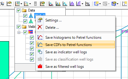 {width="4.40625in" height="2.71875in"}]
[Behavior depends on three factors:]
[·DF visible;]
[·ata coloring;]
[·enu item selected from ]{.underline}[Control data]{.underline}[ drop down button.]
[1.Plot CDF]{.underline}
[Before exporting a CDF to Petrel it must be visible on the histogram. The CDFs are selected from the ]{.underline}[Control CDFs]{.underline}[ dropdown menu. The options in here will depend on the ]{.underline}[Color data by]{.underline}[ options selected :]
[
 {width="2.6666666666666665in" height="1.4895833333333333in"}]
[CDF options for colored by datasets.]{.underline}
[
 {width="2.8541666666666665in" height="1.7395833333333333in"}]
[CDF options for colored by data visibility (Facies in this case).]{.underline}
[2.Colored by Data:]{.underline}
[
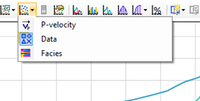 {width="3.03125in" height="1.53125in"}]
[In this case only the ]{.underline}[Data]{.underline}[ folder menu item and sub menus of this item (the datasets) from the ]{.underline}[Control data]{.underline}[ drop down will have their ]{.underline}[Save CDFs to Petrel function]{.underline}[ enabled.]
[
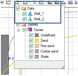 {width="2.71875in" height="2.65625in"}]
[From a dataset menu item (eg Well_1), the CDF for that dataset, if visible on the histogram (ticked) and displaying its CDF (ticked under ]{.underline}[Control CDFs]{.underline}[) will be saved as a Petrel function.]
[From the ]{.underline}[Data]{.underline}[ folder menu item, all dataset sub menus that are visible (ticked) and displaying their CDF (ticked under ]{.underline}[Control CDFs]{.underline}[) , will be saved to Petrel functions.]
[Colored]{.underline}[ by Data Visibility]{.underline}
[
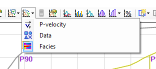 {width="3.25in" height="1.4375in"}]
[When the data is colored by a data visibility set (in this case Facies), only the ]{.underline}[Visibility]{.underline}[ folder menu item and its grandchild (the items beneath Facies, which we will call data visibility indices, ]{.underline}[Undefined]{.underline}[, ]{.underline}[Sand]{.underline}[, etc) submenu items will have their ]{.underline}[Save CDFs to Petrel functions]{.underline}[ enabled. The Facies menu item does not have a context menu.]
[
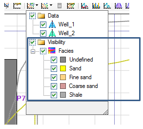 {width="3.0520833333333335in" height="2.75in"}]
[Clicking ]{.underline}[Save CDFs to Petrel functions ]{.underline}[from any data visibility index that is visible on the histogram (ticked) and ticked under ]{.underline}[the Control CDFs]{.underline}[ drop down menu will save the CDF of that index to a Petrel function.]
[Clicking ]{.underline}[Save CDFs to Petrel functions ]{.underline}[from the ]{.underline}[Visibility]{.underline}[ folder menu item will save the CDFs of all the data visibility indices that are ticked (visible on the plot), and also ticked under the ]{.underline}[Control CDFs]{.underline}[ drop down menu.]
[CDF lines may be saved to Petrel functions via right click context menus on the ]{.underline}[Control CDFs]{.underline}[ drop button:]
[
{width="2.8541666666666665in" height="1.7395833333333333in"}][
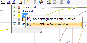 {width="3.875in" height="1.9375in"}]
[In this case on single CDFs may be saved each time. There is no option to save all CDFs at the same time, this may only be done under the ]{.underline}[Control data]{.underline}[ drop down menus]
[Multi-dimension histograms]{.underline}
[Multi-dimension histograms allows multiple histogram to be displayed in the histogram window. This allows a good understanding to be gained of how the different data is distributed across the dimensions.]
[The multi histogram view is enabled by toggling the
 {width="0.1875in" height="0.19791666666666666in"} toolbar button. ]
[
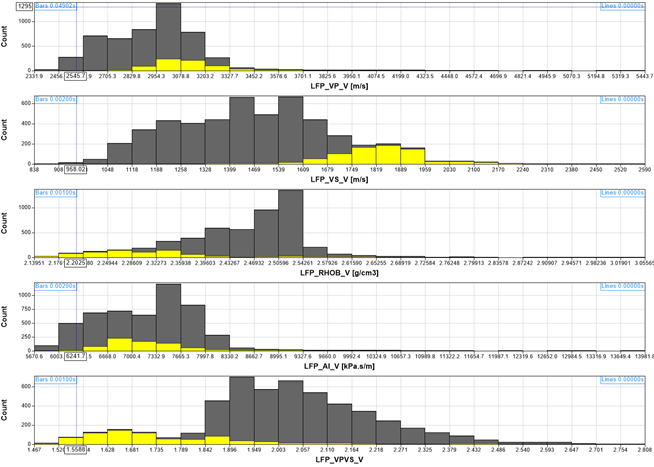 {width="6.197916666666667in" height="4.416666666666667in"}]
[The dimensions that are displayed can be selected by the ]{.underline}[Show dimension toolbar ]{.underline}[button in the same way as in Matrix and Parallel Coordinate Plot window.]
[
 {width="1.8020833333333333in" height="1.4791666666666667in"}]
[Discrete plots]{.underline}
[The following image shows a standard histogram separated into facies discrete plots and colored by dataset:]
[
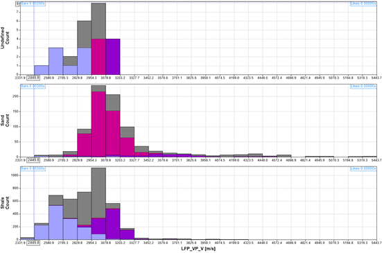 {width="5.739583333333333in" height="3.8020833333333335in"}]
[The following image shows a multi-dimension histogram separated into facies discrete plots and colored by dataset:]
[
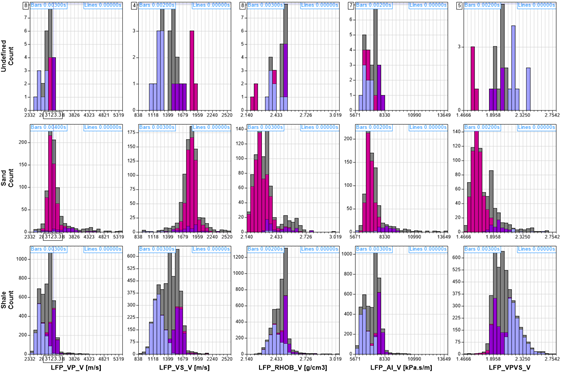 {width="5.875in" height="3.8958333333333335in"}]
[Bar charts]{.underline}
[The bar chart option provides visualization of discrete histograms. This is only possible in the histogram window.]
[A bar chart is a non-continuous histogram where each bar (or group of bars) represents a single discrete option. The bar chart count axis can show a number of different options about how the samples within each bar are combined. The default is the count of the samples.]
[
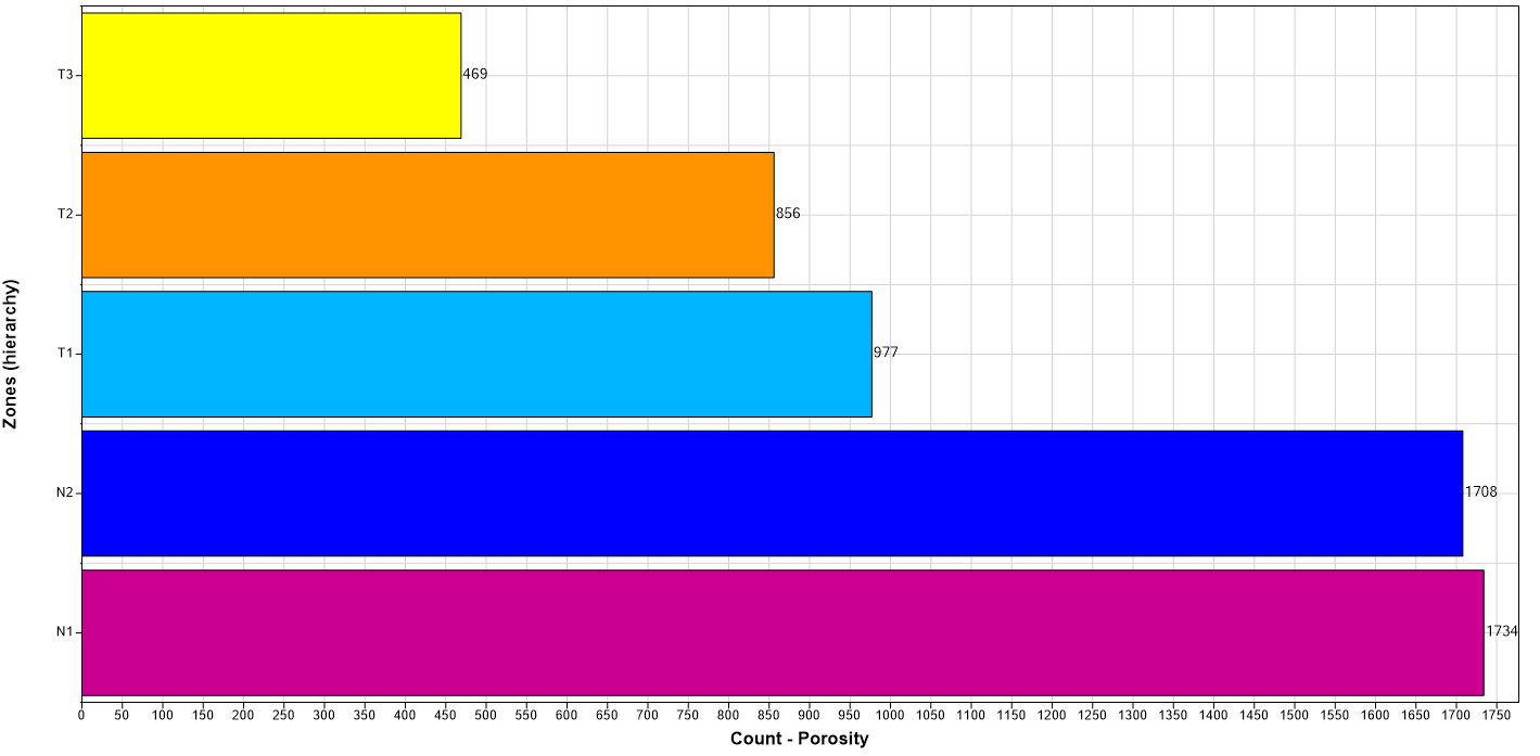 {width="6.197916666666667in" height="3.0416666666666665in"}]
[The bar chart can show any statistic value available from within Blueback Investigator. In the following example, the bar chart shows the mean porosity value of each zone within each facies.]
[ ]
[
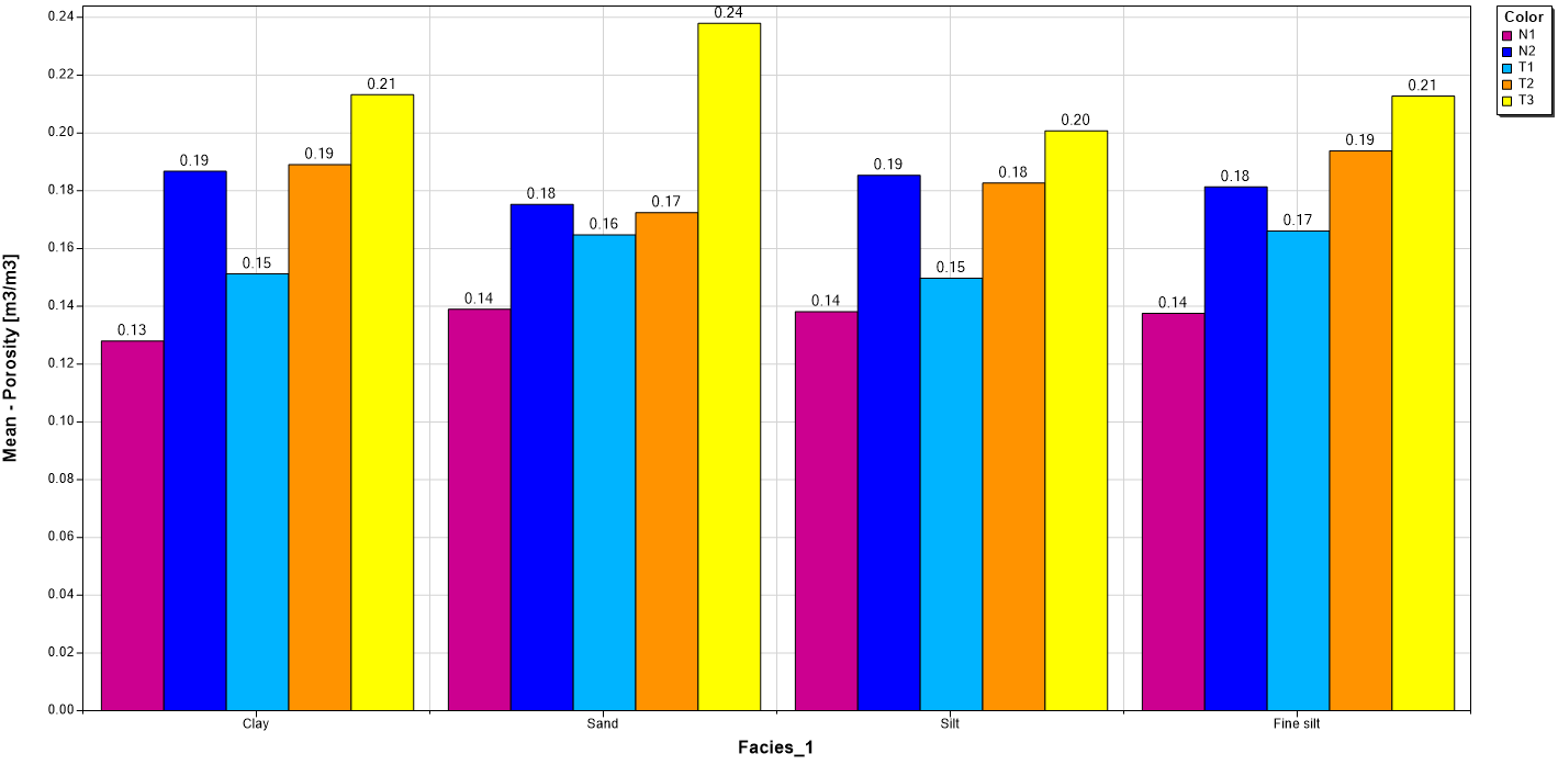 {width="6.197916666666667in" height="3.0416666666666665in"}]{.underline}
[The bar chart can also be separated by dataset. This allows the different datasets to be compared in the plot. In the following example, the bar chart shows the delta (or range of) porosity value of each facies within each zone separated by dataset. The lighter bar is the upscaled dataset and the darker bar is the grid dataset.]
[
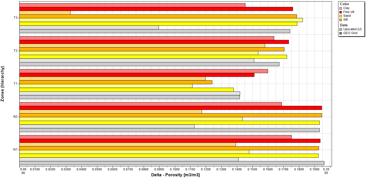 {width="6.197916666666667in" height="3.0416666666666665in"}]
[A similar plot to the above could be achieved using the discrete plot option.]
[
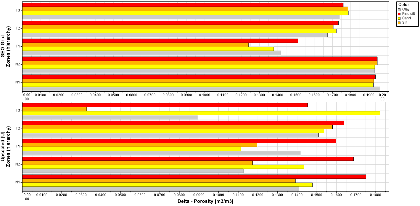 {width="6.197916666666667in" height="3.0416666666666665in"}]{.underline}
[Pie charts]{.underline}
[The pie chart option provides visualization of discrete histograms. This is only possible in the histogram window. Pie charts are an alterative representation of bar charts]{.underline} and should be setup in the same way.
[The rendering option can be toggled between bar charts and pie charts using this toolbar button ]
[The following example, shows a pie chart per zone each showing the mean porosity within each facies.]
[
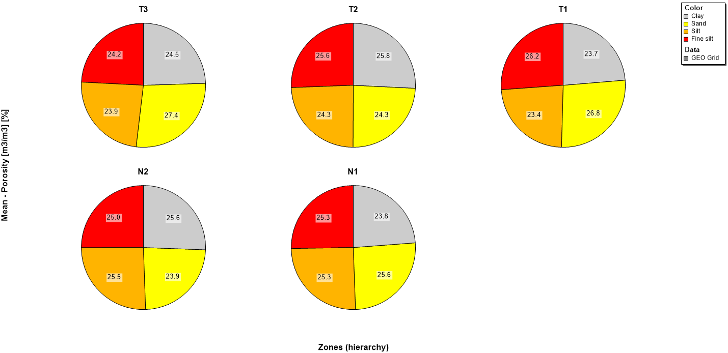 {width="6.197916666666667in" height="3.0104166666666665in"}]
[Rose diagram]{.underline}
[Blueback Investigator supports enhanced visualisation of angular data (eg rose diagrams and angular scatterplots). ]
[This is principally useful for analysis of dip and/or azimuth data. A rose diagram will be automatically used whenever a histogram is displayed is based on templates that use a rotation unit measurement (eg radians/degrees). All features of Investigator and fully integrated with these new visualisations.]
[The crosshair shown on angular plots will indicate the angle using a radius line with the value labeled on the circumference of the plot. The magnitude value will be indicated by a crosshair circle with the value labeled on the horizontal or vertical axis (dependent on the plot). The magnitude at the center of the plot is the minimum value on the axis and the magnitude at the circumference is the maximum value on the axis. ]
[This image is an example of a rose diagram displayed in a histogram window.]
[
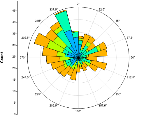 {width="5.145833333333333in" height="4.510416666666667in"}]
[Rank-Percentile analysis]{.underline}
[The rank percentile analysis option provides a visualization option to compare different datasets. This is only possible in the histogram window.]
[Rank-percentile analysis is enabled via the Show data toolbar menu.]
[
 {width="2.71875in" height="0.8541666666666666in"}]
[The statistic and dimension being compared can be selected via these toolbar options:]
[
 {width="0.8645833333333334in" height="0.5104166666666666in"}]
[The plot and table visualize the chosen statistic and dimension for each dataset. The discrete data included in each dataset can be selected in the control tree. THis allows the data to be combined based on zones, segments, facies and boundaries as required. A CDF is plotted over the bars showing the cumulative distribution of the datasets.]
[
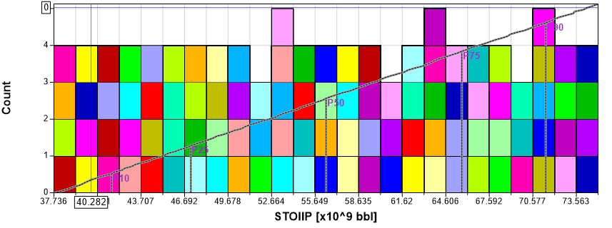 {width="6.197916666666667in" height="2.3125in"}]
[Below the plot, a table shows the plotted data including the rank and percentile for each dataset. This table also includes all the variables used to calculate each dataset.]
[
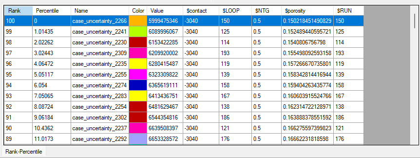 {width="6.197916666666667in" height="2.3229166666666665in"}]
[Crossplot]{.underline}
[The crossplot window is a multiple viewport window that combines a scatterplot with optional horizontal and/or vertical histograms representing the distribution of horizontal data and vertical data respectively.]
[The crossplot window allows the user to analyze two dimensions in one plot. Point coloring is used to visualize a third dimension. ]
[The plot can display any of the defined data dimensions against any other data dimensions, e.g. X against Y, Y against Z etc. It is possible to color the points in various different ways to allow the plot to show addition information. Points can be colored by both discrete and continuous dimensions.]
[The user has complete control of the symbol size and shape used for each dataset allowing the plot to provide additional information about the shown points. ]
[Points can also be binned to display a point density image behind the points.]
[In the scatterplot, the user can add selections to exclude outliers from the valid points. The valid points can then be used to determine best fit lines and these will be stored within the investigation.]
[The user also has the option to annotate the plot as necessary to add notes.]
[A crossplot window is a multiple viewport window that combines a scatterplot with horizontal and vertical histograms representing the distribution of horizontal data and vertical data respectively.]
[The ranges and data displayed in the different plot viewports is always synchronized.]
[
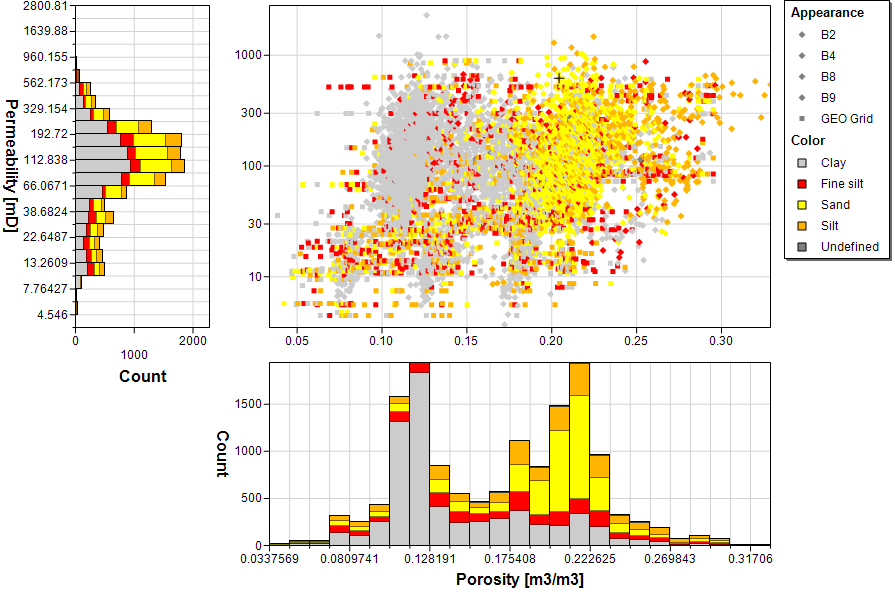 {width="6.197916666666667in" height="4.114583333333333in"}]
[Note: The axis ticks on the histograms are set by the bin size, so they may be different to the ticks on the scatterplot.]
[Discrete plots]{.underline}
[In the crossplot window it is possible to toggle between discrete plots with a common left axis or a common horizontal axis using the Toggle discrete direction (
 {width="0.21875in" height="0.2604166666666667in"}) toolbar button. This can be very helpful if wanting to compare discrete data by depth for example.]
[The following image shows a crossplot with a common left axis separated into facies discrete plots and colored by a dimension:]
[
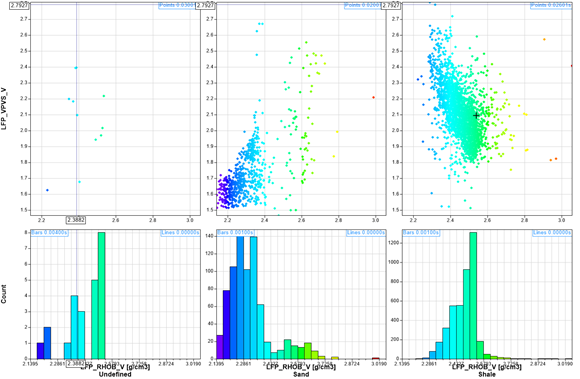 {width="6.041666666666667in" height="3.9479166666666665in"}]
[The following image shows a crossplot with a common horizontal axis separated into facies discrete plots and colored by a dimension:]
[
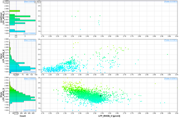 {width="6.197916666666667in" height="4.0625in"}]
[Angular plot]{.underline}
[Blueback Investigator supports enhanced visualisation of angular data (eg rose diagrams and angular scatterplots). ]
[This is principally useful for analysis of dip and/or azimuth data. An angular scatterplot will be automatically used whenever a scatterplot is displayed is based on templates that use a rotation unit measurement (eg radians/degrees). All features of Investigator and fully integrated with these new visualisations.]
[The crosshair shown on angular plots will indicate the angle using a radius line with the value labeled on the circumference of the plot. The magnitude value will be indicated by a crosshair circle with the value labeled on the horizontal or vertical axis (dependent on the plot). The magnitude at the center of the plot is the minimum value on the axis and the magnitude at the circumference is the maximum value on the axis. ]
[This image is an example of an angular scatterplot displayed in a crossplot window.]
[
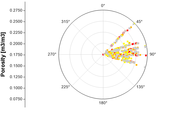 {width="6.197916666666667in" height="4.083333333333333in"}]
[Matrix]{.underline}
[A matrix plot combines several dimensions of data into one single plotting window. The plot is a combination of histograms and scatterplots. The plotting window supports selections, annotations, contours and much more.]
[When an investigation is initially displayed in a matrix window, only the first 5 continuous dimensions will be shown. Additional dimensions can be added removed using this toolbar button.]
[
 {width="1.6875in" height="1.375in"}]
[The viewports are linked together so a zoom/selection in the window will take effect in other windows as well.]
[
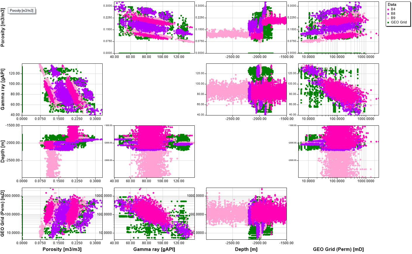 {width="6.197916666666667in" height="3.8229166666666665in"}]
[The area in the Permeability/Porosity plot is filtered. Inactive points (outside of filter) are marked light brown (from the filter color). A small cross indicates the relationship of the picked point in the other plotted dimensions.]
[Support for equations]
[Best fit equations can be created from the matrix window via the scatterplot context menu. Right click within the required scatterplot and select the desired equation.]
[Equations visible in the matrix window will be drawn in all scatterplots in which the equation is valid. This means the equation will appear in at least two scatterplots. Blueback Rock Physics supports transforming Rock Physics Models into different elastic spaces and therefore it is possible to display some RPMs in multiple scatterplots depending on the displayed dimensions.]
[Discrete plots]{.underline}
[When a matrix plot is displayed as discrete plots then the first row of plots is repeated for each separate discrete data group.]
[The following image shows a matrix window separated into facies discrete plots and colored by dataset:]
[
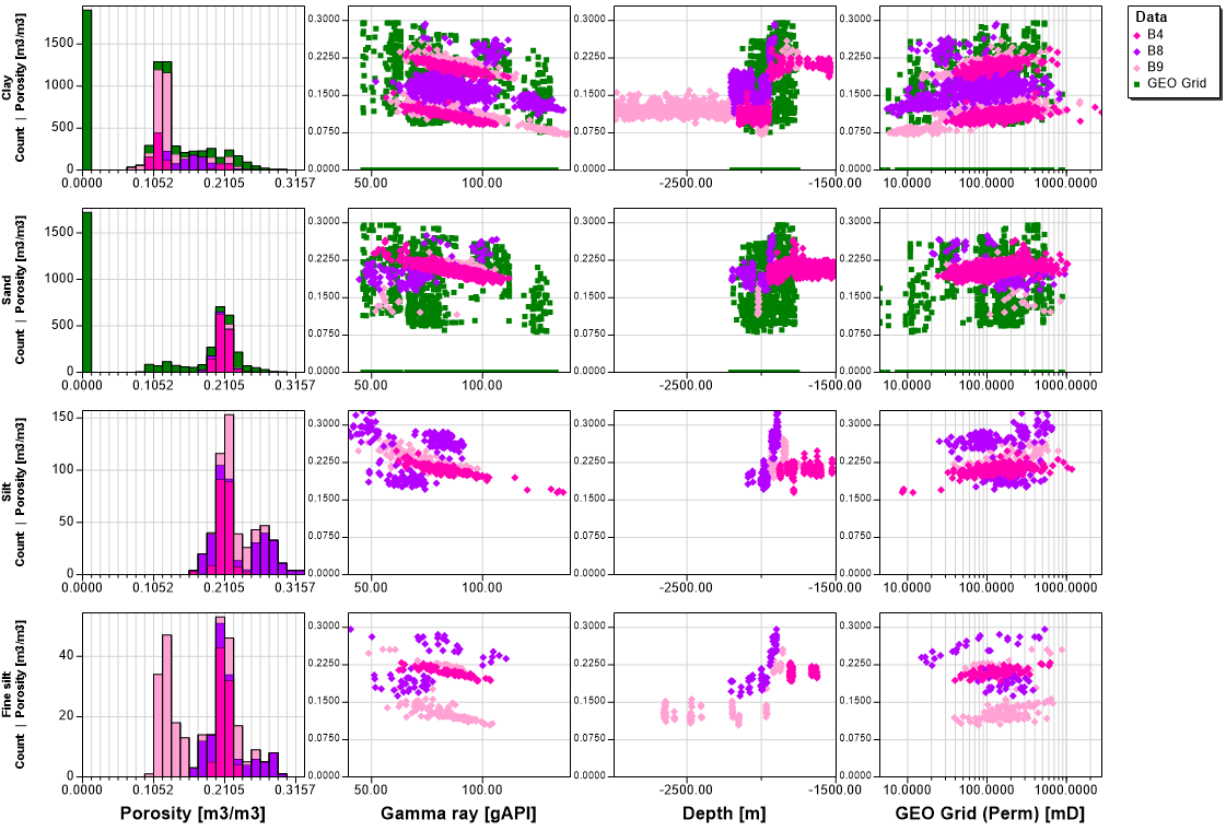 {width="6.197916666666667in" height="4.197916666666667in"}]
[Angular plots]{.underline}
[A investigation that contains both linear and angular dimension data will mix cartesian and angular plots on the matrix window. ]
[This image is an example of a mixed linear and angular data displayed in a matrix window.]
[
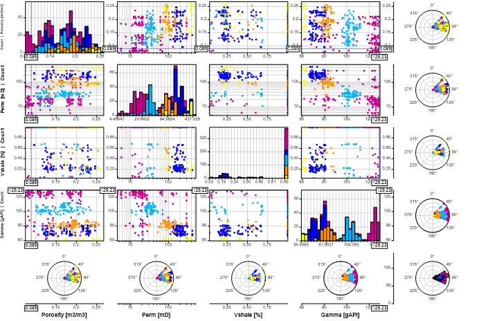 {width="6.197916666666667in" height="4.145833333333333in"}]
[Opening Linked Windows]{.underline}
[The context menu shown within a matrix window viewport allows the users to quickly and easily create a dedicated histogram or crossplot window from an existing viewport. This is very useful when exploring data in the matrix plot and wanting to drill further into specifics. ]
[The new window is automatically linked to the original window and will update when either control tree or viewport ranges are changed in either window.]
[The new window can be disconnected from the original by deselecting the link toolbar buttons.]
[Parallel coordinates]{.underline}
[The Parallel coordinates plot (PCP) window is used to identify trends in n-dimensional data.]
[
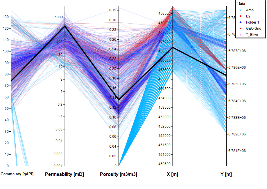 {width="6.197916666666667in" height="4.375in"}]
[Generally speaking, the more the lines in the plot form horizontal stacked parallel lines the more the dimensions correlate. This also indicates that it might be possible to predict one dimension from another. The PCP window supports color by discrete value, 1d selections, cross window picking of points (Black line above is a picked point in another plot.) and much more.]
[Data decimation]{.underline}
[For visualization purposes the PCP window decimates the data in the display. ]
[The PCP window:]
[displays approximately 1000 lines per investigation point weighted by the dataset]
[uses every n'th sample from investigation dataset based on fraction needed (1000/total points)]
[Outliers are also taken into account. Every n'th point in the investigation is considered, but outliers are also recorded. This means that there will potentially be more than 1000 lines (points from the investigation) in the display.]
[Further reading]{.underline}
[For more information on the PCP and its potential uses see this wikipedia article]{.underline}.
[Discrete plots]{.underline}
[The following image shows a parallel coordinates window separated into facies discrete plots and colored by dataset:]
[
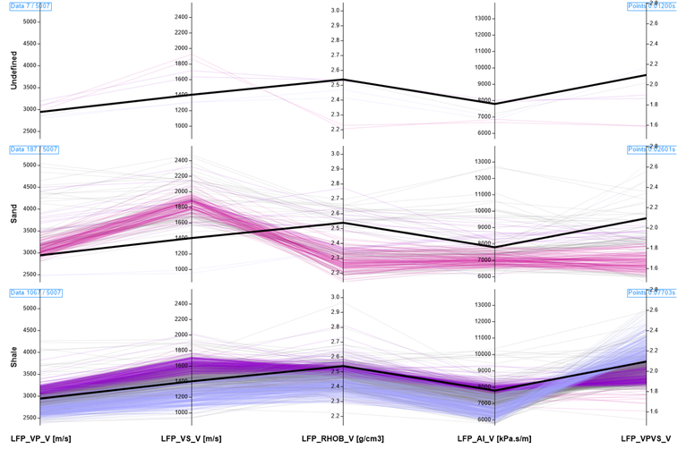 {width="6.197916666666667in" height="4.0625in"}]
[Time series]{.underline}
[The time series window is used to display time series data. The plots will always have a horizontal date axis.]
[As all data displayed in the plot has a common date dimension, it is possible to display multiple dimensions all on the same plot with multiple axes on either the left or right of the plot. This allows relationships between different dimensions to be more easily identified.]
[The time series window has an option to show displayed data either colored by or using appearance selected for each dimension.]
[The statistics shown for a fan dataset will be those of the P50 statistics from the fan.]
[
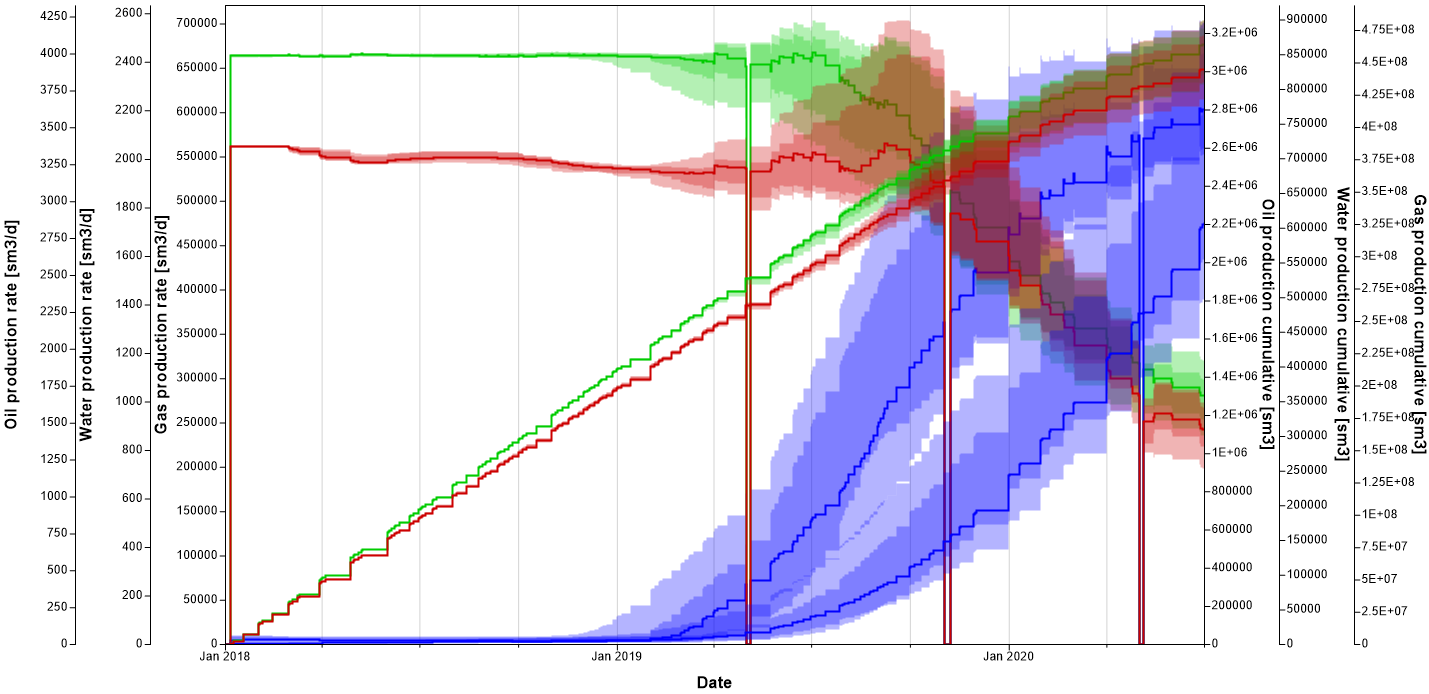 {width="6.197916666666667in" height="3.0104166666666665in"}]
[The plot can be easily toggled to show separate plots if more clarity is needed.]
[
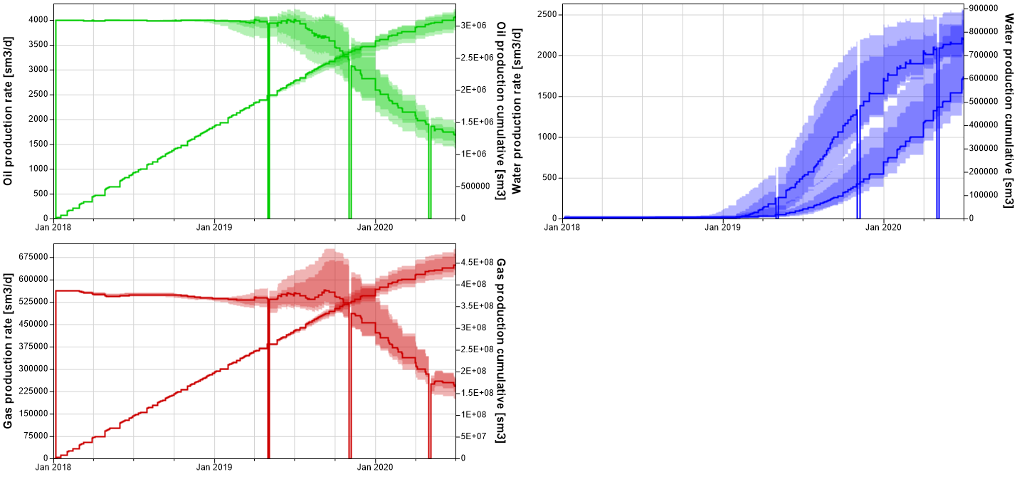 {width="6.197916666666667in" height="3.0104166666666665in"}]
[Multiple summary identifiers can also be shown either on the same plot or on separate plots with a single toggle.]
[
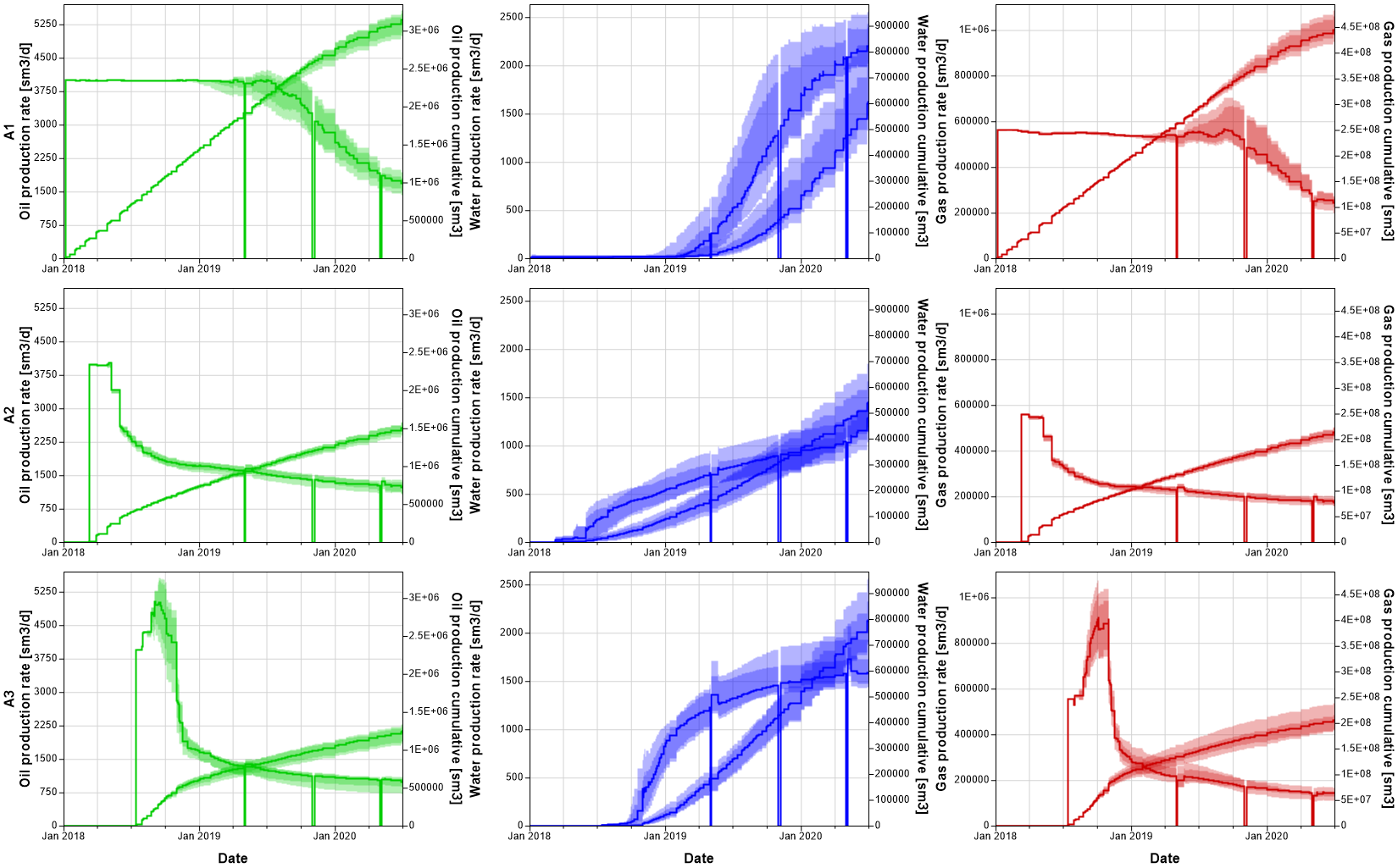 {width="6.197916666666667in" height="3.84375in"}]
[Blueback Investigator 3D plot]{.underline}
[The Blueback Investigator 3D plot window allows the user to view investigations in 3D conceptual and or real world space. The 3D plot allows the user to view the conceptual space for various directions which can help understand the relationships between the different dimensions.]
[Note: The 3D plot only support basic manipulation of the view. Adding selections etc should be performed on the histogram and scatterplot viewports.]
[
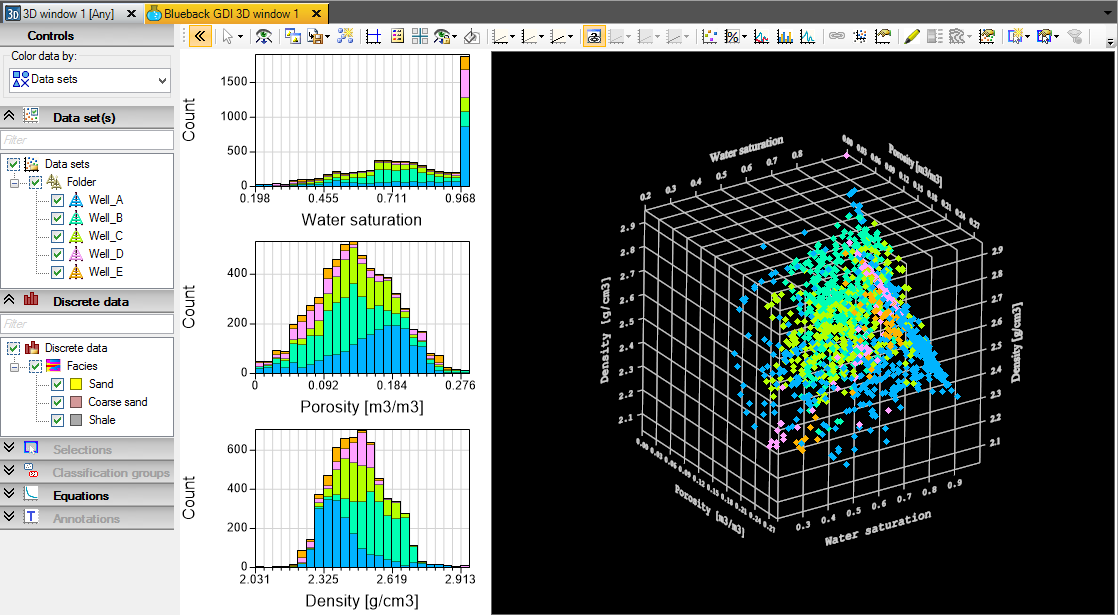 {width="6.197916666666667in" height="3.3958333333333335in"}]
[The 3 viewports on the left of the plot window can show either histograms as above or scatterplots as shown below. It is also possible to display different dimension in the 3D plot compared to the histograms/scatterplots. This effectively allows the user to visualize up to 7 different dimension at a time.]
[
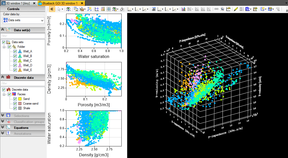 {width="6.197916666666667in" height="3.3854166666666665in"}]
[Petrel 3D window]{.underline}
[It is possible to view spatial investigations in the Petrel 3D window. A spatial investigation must contain the spatial X, Y dimension and at least the time or depth dimension.]
[
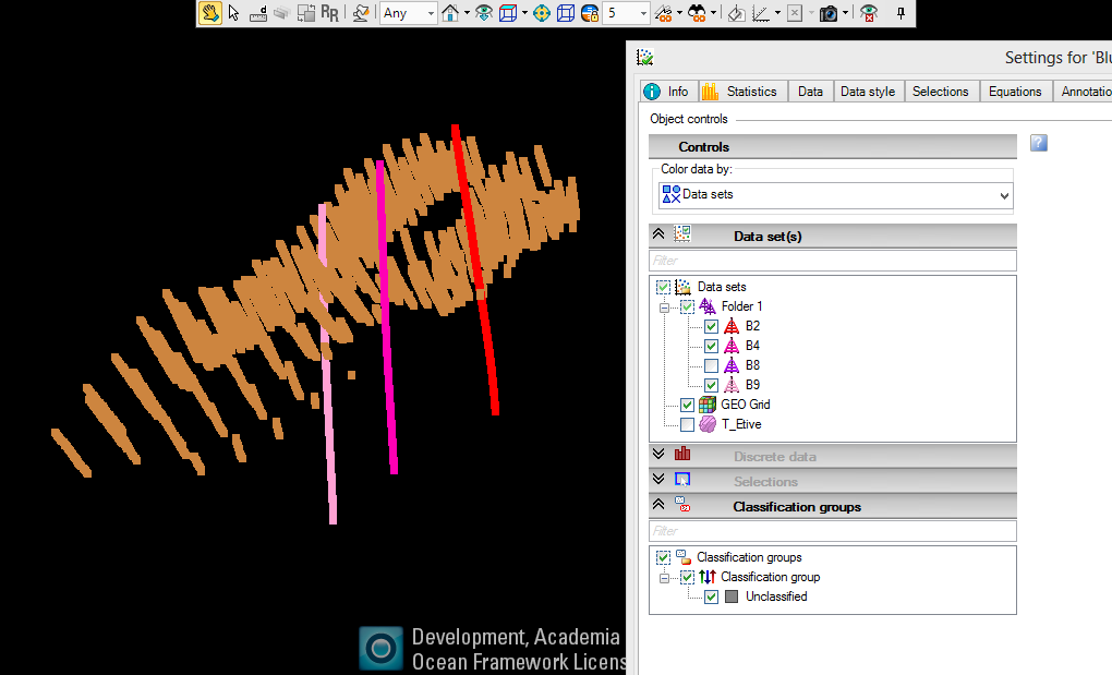 {width="6.197916666666667in" height="3.7604166666666665in"}]
[How and what is displayed in the 3D window is controlled via the Style 3D tab]{.underline} in the investigation settings dialog.
[Petrel map window]{.underline}
[It is possible to view spatial investigations in the Petrel map window. A spatial investigation must contain the spatial X, Y dimension and at least the time or depth dimension.]
[
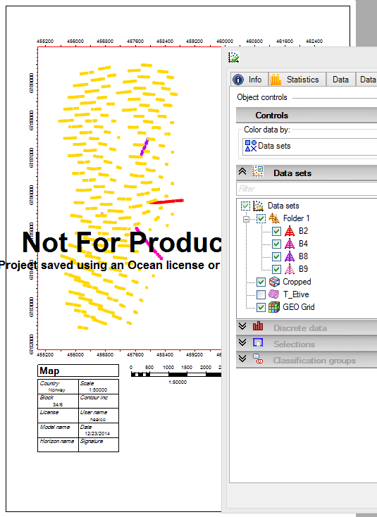 {width="5.572916666666667in" height="7.645833333333333in"}]
[How and what is displayed in the map window is controlled via the Petrel window style]{.underline} in the investigation settings dialog.
[Petrel seismic windows]{.underline}
[It is possible to view spatial investigations in the Petrel seismic windows. A spatial investigation must contain the spatial X, Y dimension and at least the time or depth dimension.]
[
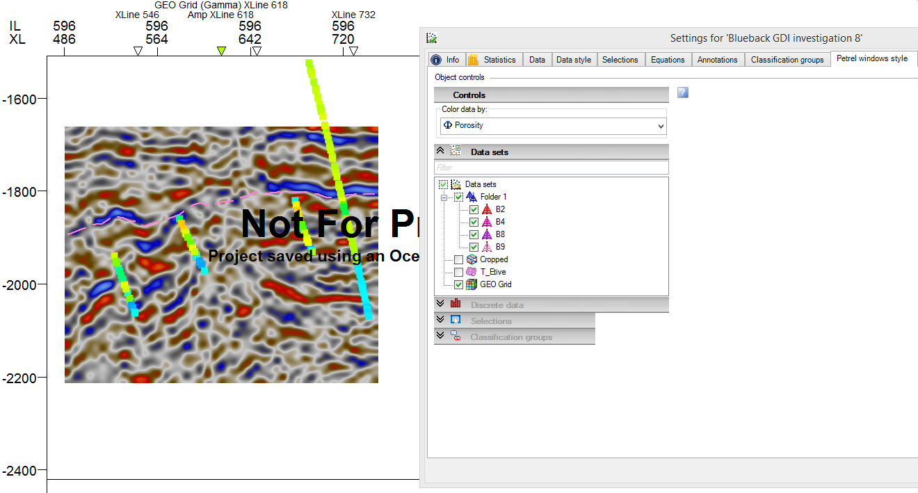 {width="6.197916666666667in" height="3.3333333333333335in"}]
[How and what is displayed in the window is controlled via the Petrel window style tab]{.underline} in the investigation settings dialog.
[Petrel well section window]{.underline}
[It is possible to view spatial investigations in the Petrel well section window. A spatial investigation must contain the spatial X, Y dimension and at least the time or depth dimension.]
[
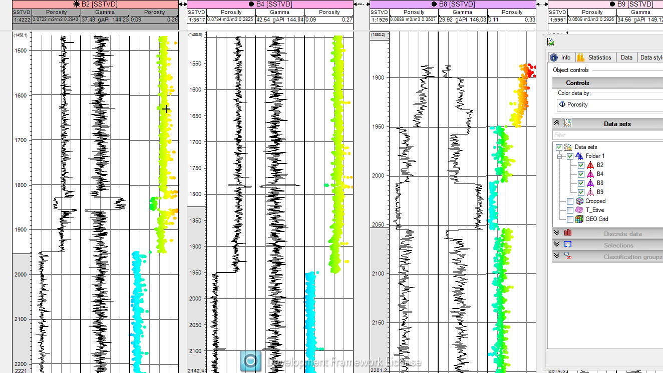 {width="6.197916666666667in" height="3.4791666666666665in"}]
[How and what is displayed in the Petrel window is controlled via the Petrel window style tab]{.underline} in the investigation settings dialog.
[Toolbars]{.underline}
[The basic functionality for each of the Blueback Investigator plots is driven from the toolbars in the plot windows.]
[General]{.underline}
[
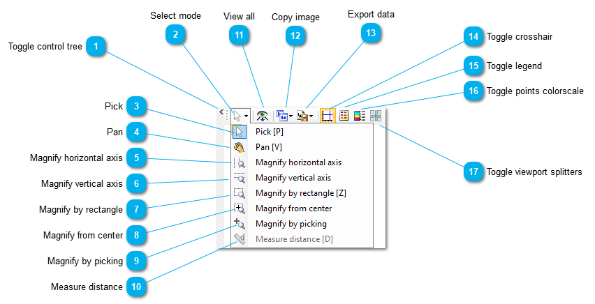 {width="6.197916666666667in" height="3.1666666666666665in"}]
[
 {width="0.4166666666666667in" height="0.4166666666666667in"}]{.underline}[Toggle control tree]{.underline}
[
 {width="0.15625in" height="0.2916666666666667in"}]
[Toggles visibility of the window control tree.]
[
 {width="0.4166666666666667in" height="0.4166666666666667in"}]{.underline}[Select mode]{.underline}
[
 {width="0.3333333333333333in" height="0.2708333333333333in"}]
[Displays the active mouse mode. Clicking it displays the mode drop down menu. ESC toggles between current mode and last used mode.]
[Scroll zoom options are available using the middle mouse button. No need to change the mode to activate.]{.underline}
[
 {width="0.4166666666666667in" height="0.4166666666666667in"}]{.underline}[Pick]{.underline}
[
 {width="0.25in" height="0.2604166666666667in"}]
[Use the mouse to pick points in the plot. Shortcut key is P.]
[
 {width="0.4166666666666667in" height="0.4166666666666667in"}]{.underline}[Pan]{.underline}
[
 {width="0.1875in" height="0.22916666666666666in"}]
[Use the mouse to pan the visible plot area. Shortcut key is V.]
[
 {width="0.4166666666666667in" height="0.4166666666666667in"}]{.underline}[Magnify horizontal axis]{.underline}
[
 {width="0.21875in" height="0.21875in"}]
[Magnify the plot horizontally by clicking and dragging to define an area of interest.]
[Only zoom option available in the histogram window.]{.underline}
[
 {width="0.4166666666666667in" height="0.4166666666666667in"}]{.underline}[Magnify vertical axis]{.underline}
[
 {width="0.2916666666666667in" height="0.21875in"}]
[Magnify the plot vertically by clicking and dragging to define an area of interest.]
[
 {width="0.4166666666666667in" height="0.4166666666666667in"}]{.underline}[Magnify by rectangle]{.underline}
[
 {width="0.19791666666666666in" height="0.22916666666666666in"}]
[Magnify the plot by clicking and dragging using the left mouse button to draw a rectangular area of interest. Shortcut key is Z.]
[Available only from the scatterplot, crossplot and matrix plot windows.]{.underline}
[
 {width="0.4166666666666667in" height="0.4166666666666667in"}]{.underline}[Magnify from center]{.underline}
[
 {width="0.1875in" height="0.22916666666666666in"}]
[Magnify the plot by clicking and dragging to draw a rectangular area of interest centered around the mouse click point.]
[Available only from the scatterplot, crossplot and matrix plot windows.]{.underline}
[
 {width="0.4166666666666667in" height="0.4166666666666667in"}]{.underline}[Magnify by picking]{.underline}
[
 {width="0.22916666666666666in" height="0.22916666666666666in"}]
[Magnify the plot using the left mouse button to zoom in around the point clicked or the right mouse button to zoom out. The zoom in/out can be continued by holding down the mouse buttons.]
[Available only from the scatterplot and crossplot windows.]{.underline}
[
 {width="0.4166666666666667in" height="0.4166666666666667in"}]{.underline}[Measure distance]{.underline}
[
 {width="0.25in" height="0.25in"}]
[The Measure distance tool is covered in the X, Y, Time and Depth plots]{.underline} section.
[
 {width="0.4166666666666667in" height="0.4166666666666667in"}]{.underline}[View all]{.underline}
[
 {width="0.23958333333333334in" height="0.20833333333333334in"}]
[Reset the magnification so that all the data points are visible. If the axis min/max values have been set manually in the axis settings view all will use these values, else the min/max of the dataset will be used.]
[
 {width="0.4166666666666667in" height="0.4166666666666667in"}]{.underline}[Copy image]{.underline}
[
 {width="0.3125in" height="0.21875in"}]
[When clicking ]{.underline}[Copy image]{.underline}[, the following options are displayed:]
[
 {width="2.3229166666666665in" height="0.7291666666666666in"}]
[Copy bitmap ]{.underline}[- Copy the current window to the clipboard as a bitmap image]
[Copy enhanced metafile]{.underline}[ - Copy the current window to the clipboard as an enhanced metafile]
[
 {width="0.4166666666666667in" height="0.4166666666666667in"}]{.underline}[Export data]{.underline}
[
 {width="0.3020833333333333in" height="0.23958333333333334in"}]
[When clicking ]{.underline}[Export data]{.underline}[, the following options are displayed:]
[
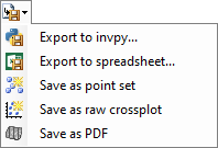 {width="2.0625in" height="1.40625in"}]
[Export to invpy]{.underline}[ produces a .invpy file that can be used to transfer a complete investigation to an InvestigatorPy python environment]
[Export to spreadsheet]{.underline}[ produces a .csv file that can be read into Excel. ]
[Save as point set]{.underline}[ creates a static point set in the input tree.]
[Save as raw crossplot ]{.underline}[saves a Petrel raw crossplot object in the input tree. This object contains the current plotted dimension points and can be used in property modeling workflows. It can be displayed in the Function window.]
[Save as PDF]{.underline}[ saves a 2D probability density function onto a Petrel surface with attributes (Z, PDF, X and Y). This can be used in the ]{.underline}[Blueback Rock Physics]{.underline}[ product.]
[See Export options]{.underline} for more information.
[
 {width="0.4166666666666667in" height="0.4166666666666667in"}]{.underline}[Toggle crosshair]{.underline}
[
 {width="0.25in" height="0.23958333333333334in"}]
[Use this option to turn on and off the crosshair in the window.]
[
 {width="0.4166666666666667in" height="0.4166666666666667in"}]{.underline}[Toggle legend]{.underline}
[
 {width="0.22916666666666666in" height="0.22916666666666666in"}]
[Shows or hides the legend.]
[
 {width="0.4166666666666667in" height="0.4166666666666667in"}]{.underline}[Toggle points colorscale]{.underline}
[
 {width="0.2604166666666667in" height="0.2916666666666667in"}]
[Shows of hides the points color scale.]
[
 {width="0.4166666666666667in" height="0.4166666666666667in"}]{.underline}[Toggle viewport splitters]{.underline}
[
 {width="0.2604166666666667in" height="0.2916666666666667in"}]
[Clicking on this button allows the sizes of the plots in the window to be changed by dragging the blue lines.]
[Available only from the crossplot window.]{.underline}
[
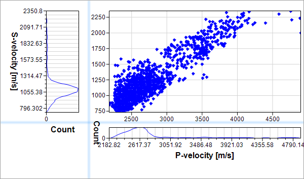 {width="4.739583333333333in" height="2.7916666666666665in"}]
[Data]{.underline}
[Options to control how the data is displayed.]
[
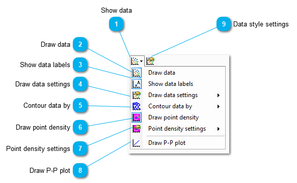 {width="6.072916666666667in" height="3.75in"}]
[ ]
[
{width="0.4166666666666667in" height="0.4166666666666667in"}]{.underline}[Show data]{.underline}[
 {width="0.28125in" height="0.22916666666666666in"}]
[Displays the submenu as shown.]
[
{width="0.4166666666666667in" height="0.4166666666666667in"}]{.underline}[Draw data]{.underline}[
 {width="0.2916666666666667in" height="0.2916666666666667in"}]
[Display/hide the data points from the plot]
[
{width="0.4166666666666667in" height="0.4166666666666667in"}]{.underline}[Show data labels]{.underline}[
 {width="0.2916666666666667in" height="0.2916666666666667in"}]
[Display/hide dataset labels above each data point in the plot.]
[Note: Toggling labels when lots of data points are shown in the plot will fill the plot with labels and can make it unusable. ]
[
{width="0.4166666666666667in" height="0.4166666666666667in"}]{.underline}[Draw data settings]{.underline}[
 {width="0.2708333333333333in" height="0.2604166666666667in"}]
[Shows the draw data settings submenu:]
[
 {width="1.8020833333333333in" height="0.53125in"}]
[Toggle decimation]{.underline}[ option controls whether plotted data is decimated. Decimation will reduce the number of rendered all points if points are close together.]
[Overplot data ]{.underline}[option controls whether all points that are drawn on a particular pixel are rendered or just the point from the dataset with the best priority.]
[
{width="0.4166666666666667in" height="0.4166666666666667in"}]{.underline}[Contour data by]{.underline}[
 {width="0.22916666666666666in" height="0.19791666666666666in"}]
[Displays a submenu to control contouring of point densities:]
[
 {width="1.4791666666666667in" height="1.03125in"}]
[See Contouring data]{.underline} for more information.
[
{width="0.4166666666666667in" height="0.4166666666666667in"}]{.underline}[Draw point density]{.underline}[
 {width="0.23958333333333334in" height="0.23958333333333334in"}]
[Toggles display of the point density plot for the data.]
[
{width="0.4166666666666667in" height="0.4166666666666667in"}]{.underline}[Point density settings]{.underline}[
 {width="0.25in" height="0.21875in"}]
[If data is plotted by point density, then this shows a submenu which controls options for the point density plot]
[
 {width="2.5208333333333335in" height="0.5in"}]
[Toggle empty point density bins]{.underline}[ option controls whether empty 'bins' should be colored (below left) or not (below right).]
[Toggle point density color scale]{.underline}[ option controls whether the colorscale shows information for the point density or from the selected continuous dimension.]
[Available only from the scatterplot, crossplot and matrix windows.]{.underline}
[
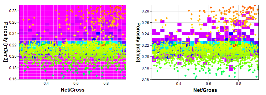 {width="6.197916666666667in" height="2.21875in"}]
[
{width="0.4166666666666667in" height="0.4166666666666667in"}]{.underline}[Draw P-P plot]{.underline}[
 {width="0.2604166666666667in" height="0.28125in"}]
[Toggles between a normal data plot and a percentile plot. ]
[See Percentile-Percentile plots]{.underline} for more information.
[
{width="0.4166666666666667in" height="0.4166666666666667in"}]{.underline}[Data style settings]{.underline}[
 {width="0.23958333333333334in" height="0.22916666666666666in"}]
[Opens a dialog which allows various dataset style settings to be edited.]
[Plot axes]{.underline}
[Options to control what is displayed in which plot axis.]
[
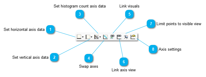 {width="6.197916666666667in" height="2.3125in"}]
[
{width="0.4166666666666667in" height="0.4166666666666667in"}]{.underline}[Set horizontal axis data]{.underline}[
 {width="0.2916666666666667in" height="0.20833333333333334in"}]
[A drop down menu which allows selection of the data to be plotted in the x-axis.]
[
 {width="1.53125in" height="1.0104166666666667in"}]
[
{width="0.4166666666666667in" height="0.4166666666666667in"}]{.underline}[Set vertical axis data]{.underline}[
 {width="0.3020833333333333in" height="0.20833333333333334in"}]
[A drop down menu which allows selection of the data to be plotted in the y-axis.]
[
 {width="1.53125in" height="1.0104166666666667in"}]
[For a histogram window, this functionality has a different icon (
 {width="0.28125in" height="0.1875in"}) . It controls whether the y-axis should display data count, percentage or weighted percentage (Model data only).]
[
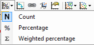 {width="1.9583333333333333in" height="0.9479166666666666in"}]
[In the crossplot window and the matrix window the histogram y-axis control button is displayed along with the horizontal and vertical axis data buttons.
 {width="0.9166666666666666in" height="0.19791666666666666in"} See Set histogram count axis data.]
[
{width="0.4166666666666667in" height="0.4166666666666667in"}]{.underline}[Set histogram count axis data]{.underline}[
 {width="0.3125in" height="0.20833333333333334in"}]
[A drop down menu which controls the display type to be plotted in the histogram count axis.]
[
{width="1.9583333333333333in" height="0.9479166666666666in"}][Weighted percentage is available for model data only.]
[Available as unique button only for crossplot and matrix windows.]{.underline}
[
{width="0.4166666666666667in" height="0.4166666666666667in"}]{.underline}[Swap axes]{.underline}[
 {width="0.22916666666666666in" height="0.20833333333333334in"}]
[Swaps the current x and y-axis selections.]
[On a histogram window this swaps the orientation of the histogram bars/lines from vertical or horizontal.]
[Available only from the histogram and crossplot windows.]{.underline}
[
{width="0.4166666666666667in" height="0.4166666666666667in"}]{.underline}[Link visuals]{.underline}[
 {width="0.2916666666666667in" height="0.2916666666666667in"}]
[Links the visible objects between windows. Changes made in the control tree of one window will affect all linked windows. This can be very useful when linking to Petrel windows.]
[This toggle option needs to be selected in each window for it to be linked. ]
[Note: only the axis ranges are linked; the data selections, visibility and other settings are not linked.]{.underline}
[
{width="0.4166666666666667in" height="0.4166666666666667in"}]{.underline}[Link axis view]{.underline}[
 {width="0.23958333333333334in" height="0.23958333333333334in"}]
[Links the axis ranges between windows. ]
[This toggle option needs to be selected in each window for it to be linked. ]
[Note: only the axis ranges are linked; the data selections, visibility and other settings are not linked.]{.underline}
[
{width="0.4166666666666667in" height="0.4166666666666667in"}]{.underline}[Limit points to visible view]{.underline}[
 {width="0.21875in" height="0.20833333333333334in"}]
[This option allows the user to limit the data displayed in the histogram to only the currently visible data. For example, with this option enabled in a crossplot window the histograms will accurately represent the distribution of the data visible in the scatterplot viewport. However, with this option disabled in a crossplot the two histograms will represent the distribution of the whole dataset, not just the points displayed on the scatterplot.]
[This functionality is primarily of use in the crossplot window, where it is disabled by default, but it also affects histogram plots if they are linked to other windows. This option is toggled off by default for histograms.]
[
{width="0.4166666666666667in" height="0.4166666666666667in"}]{.underline}[Axis settings]{.underline}[
 {width="0.21875in" height="0.20833333333333334in"}]
[Opens a dialog which allows various axis settings to be changed. ]
[
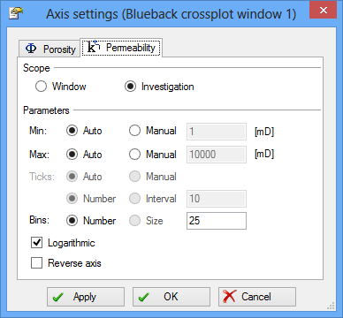 {width="4.041666666666667in" height="3.75in"}]
[Changes made in this dialog applies to the investigation by default, but can be made window specific by selecting Window as Scope. See Axis settings]{.underline} for more information.
[Discrete plots / Data highlighting]{.underline}
[Options to control the discrete plots / data highlighting applied to the window.]
[
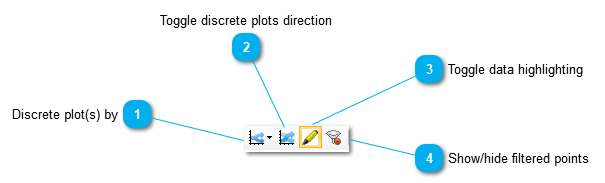 {width="6.197916666666667in" height="1.8645833333333333in"}]
[
{width="0.4166666666666667in" height="0.4166666666666667in"}]{.underline}[Discrete plot(s) by]{.underline}[
 {width="0.2916666666666667in" height="0.2916666666666667in"}]
[A dropdown menu allowing which discrete option should be used to split the plot. ]
[The displayed discrete plots are controlled by the discrete options marked visible in the control tree.]
[
 {width="1.5520833333333333in" height="1.09375in"}]
[
{width="0.4166666666666667in" height="0.4166666666666667in"}]{.underline}[Toggle discrete plots direction]{.underline}[
 {width="0.2916666666666667in" height="0.2916666666666667in"}]
[Toggles the split direction on crossplots. The plot will be repeated wither left-right or top-bottom. The different options result in a different histogram being repeated. ]
[Available as unique button only for crossplot window.]{.underline}
[
{width="0.4166666666666667in" height="0.4166666666666667in"}]{.underline}[Toggle data highlighting]{.underline}[
 {width="0.2916666666666667in" height="0.2916666666666667in"}]
[Toggle data highlighting mode on/off.]
[See Data highlighting]{.underline} for more information
[
{width="0.4166666666666667in" height="0.4166666666666667in"}]{.underline}[Show/hide filtered points]{.underline}[
 {width="0.3020833333333333in" height="0.3020833333333333in"}]
[Toggle whether filtered or unhighlighted points are displayed on not.]
[Selections]{.underline}
[Allows filters and classifications to be added and updated.]
[
 {width="4.572916666666667in" height="0.4791666666666667in"}]
[
{width="0.4166666666666667in" height="0.4166666666666667in"}]{.underline}[Add selections]{.underline}[
 {width="0.3020833333333333in" height="0.22916666666666666in"}]
[Creates a new Selection. Select one of the options from the drop down list:]
[
 {width="1.9270833333333333in" height="0.71875in"}]
[Add filter sub menu:]
[
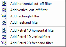 {width="2.40625in" height="1.71875in"}]
[Add classified region sub menu:]
[
 {width="2.9375in" height="0.9583333333333334in"}]
[For more information see Selections]
[
{width="0.4166666666666667in" height="0.4166666666666667in"}]{.underline}[Selection settings]{.underline}[
 {width="0.3020833333333333in" height="0.22916666666666666in"}]
[Opens a dialog which allows various selection settings to be edited:]
[
 {width="2.4375in" height="0.71875in"}]
[Equations]{.underline}
[Allows best-fit or user-defined equations to be added and updated.]
[
 {width="4.6875in" height="0.4791666666666667in"}]
[
{width="0.4166666666666667in" height="0.4166666666666667in"}]{.underline}[Add equation]{.underline}[
 {width="0.3125in" height="0.25in"}]
[Creates a new equation. Select one of the options from the drop down list:]
[
 {width="2.1979166666666665in" height="1.21875in"}]
[See Equations]{.underline} for more information.
[Available only in windows showing a scatterplot. If not in the toolbar then access via the context menu of the scatterplot.]{.underline}
[
{width="0.4166666666666667in" height="0.4166666666666667in"}]{.underline}[Equation settings]{.underline}[
 {width="0.28125in" height="0.25in"}]
[Opens a dialog which allows various equation settings to be edited.]
[Available only in windows showing a scatterplot/histogram (distributions). If not in the toolbar then access via the context menu of the scatterplot.]{.underline}
[Distributions]{.underline}
[Allows distributions to be added and updated.]
[
 {width="4.833333333333333in" height="0.4791666666666667in"}]
[
{width="0.4166666666666667in" height="0.4166666666666667in"}]{.underline}[Add distribution]{.underline}[
 {width="0.22916666666666666in" height="0.25in"}]
[Pressing the Add distribution button will open the following dialog:]
[
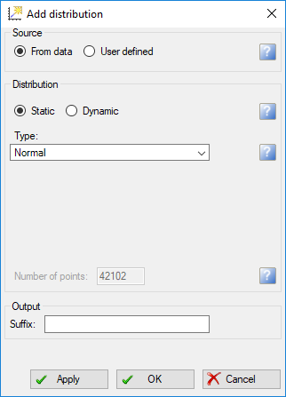 {width="3.3541666666666665in" height="4.65625in"}]
[Apply/OK creates a new distribution that is saved under "Equations".]
[See Distributions]{.underline} for more information.
[Available only in windows showing a histogram. If not in the toolbar then access via the context menu of the histogram.]{.underline}
[
{width="0.4166666666666667in" height="0.4166666666666667in"}]{.underline}[Equation settings]{.underline}[
 {width="0.21875in" height="0.21875in"}]
[Opens a dialog which allows various equation settings to be edited.]
[Available only in windows showing a histogram/crossplot (equations). If not in the toolbar then access via the context menu of the histogram.]{.underline}
[Annotations]{.underline}
[Allows annotations to be added and updated.]
[Annotations are ]{.underline}[stuck]{.underline}[ to the data so will continue to point to the same place as plots are scrolled and zoomed. Annotations are also specific to the data template space in which they have been created. This means that if the axis data selections are changed (via the
{width="0.8229166666666666in" height="0.20833333333333334in"} toolbar buttons) then the annotation will no longer appear.][
 {width="4.864583333333333in" height="0.4895833333333333in"}]
[
{width="0.4166666666666667in" height="0.4166666666666667in"}]{.underline}[Add annotation]{.underline}[
 {width="0.25in" height="0.22916666666666666in"}]
[Adds an annotation to the plot. After pressing this button, click in the plot and enter text in the dialog which appears.]
[
 {width="2.5in" height="1.2291666666666667in"}]
[
{width="0.4166666666666667in" height="0.4166666666666667in"}]{.underline}[Annotation settings]{.underline}[
 {width="0.23958333333333334in" height="0.22916666666666666in"}]
[Opens a dialog which allows annotations to be edited.]
[Statistics]{.underline}
[
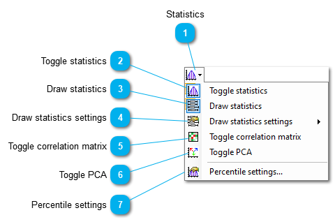 {width="5.0in" height="3.3125in"}]
[
{width="0.4166666666666667in" height="0.4166666666666667in"}]{.underline}[Statistics]{.underline}[
 {width="0.2708333333333333in" height="0.20833333333333334in"}]
[Displays the statistics submenu]
[
{width="0.4166666666666667in" height="0.4166666666666667in"}]{.underline}[Toggle statistics]{.underline}[
 {width="0.2604166666666667in" height="0.23958333333333334in"}]
[Display/hide the statistics panel.]
[
 {width="6.197916666666667in" height="0.96875in"}]
[
{width="0.4166666666666667in" height="0.4166666666666667in"}]{.underline}[Draw statistics]{.underline}[
 {width="0.25in" height="0.23958333333333334in"}]
[Toggles the display of statistics overlays. ]
[A box plot]{.underline} will be drawn in histograms and a [bag plot]{.underline} will be drawn in scatterplots.
[
{width="0.4166666666666667in" height="0.4166666666666667in"}]{.underline}[Draw statistics settings]{.underline}[
 {width="0.21875in" height="0.22916666666666666in"}]
[Shows the following submenu allowing the control of which bag plots elements are drawn.]
[
 {width="1.625in" height="0.9583333333333334in"}]
[See bag plot]{.underline} for more information.
[
{width="0.4166666666666667in" height="0.4166666666666667in"}]{.underline}[Toggle correlation matrix]{.underline}[
 {width="0.21875in" height="0.21875in"}]
[Display/hide the correlation matrix panel.]
[The correlation matrix is a table showing correlation coefficients between the displayed dimensions based on the setup of the window. ]
[The coloring gives a quick overview of how "good" the correlation is. Green is a good correlation, yellow is a weak correlation and red is a poor correlation.]
[
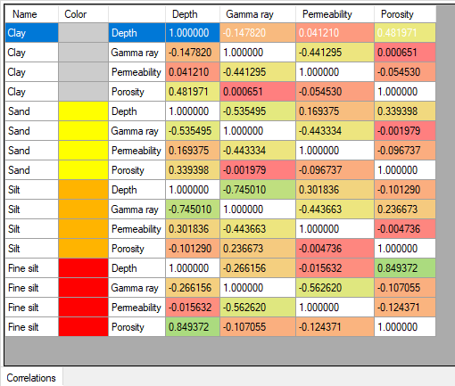 {width="5.3125in" height="4.510416666666667in"}]
[
{width="0.4166666666666667in" height="0.4166666666666667in"}]{.underline}[Toggle PCA]{.underline}[
 {width="0.23958333333333334in" height="0.21875in"}]
[Display/hide the principal component analysis]{.underline} overlay.
[
{width="0.4166666666666667in" height="0.4166666666666667in"}]{.underline}[Percentile settings]{.underline}[
 {width="0.23958333333333334in" height="0.22916666666666666in"}]
[Displays the user interface to control the displayed percentiles:]
[
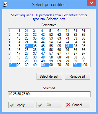 {width="3.5208333333333335in" height="4.083333333333333in"}]
[Changing the percentiles will have immediate effect in the displayed CDF's and in the histogram statistics:]
[
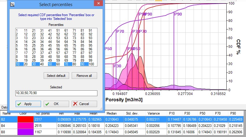 {width="6.197916666666667in" height="3.4583333333333335in"}]
[Histogram]{.underline}
[Controls how data is displayed on the histogram.]
[
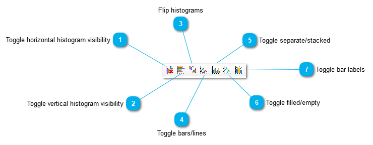 {width="6.197916666666667in" height="2.4166666666666665in"}]
[
{width="0.4166666666666667in" height="0.4166666666666667in"}]{.underline}[Toggle horizontal histogram visibility]{.underline}[
 {width="0.2916666666666667in" height="0.2916666666666667in"}]
[Toggles horizontal histogram visibility]
[
{width="0.4166666666666667in" height="0.4166666666666667in"}]{.underline}[Toggle vertical histogram visibility]{.underline}[
 {width="0.2916666666666667in" height="0.2916666666666667in"}]
[Toggles vertical histogram visibility]
[
{width="0.4166666666666667in" height="0.4166666666666667in"}]{.underline}[Flip histograms]{.underline}[
 {width="0.2916666666666667in" height="0.2708333333333333in"}]
[Toggles the histogram orientation]
[
{width="0.4166666666666667in" height="0.4166666666666667in"}]{.underline}[Toggle bars/lines]{.underline}[
 {width="0.21875in" height="0.20833333333333334in"}]
[Toggles between displaying the data as bars
 {width="0.22916666666666666in" height="0.20833333333333334in"}or lines
  {width="0.20833333333333334in" height="0.17708333333333334in"}.]
[
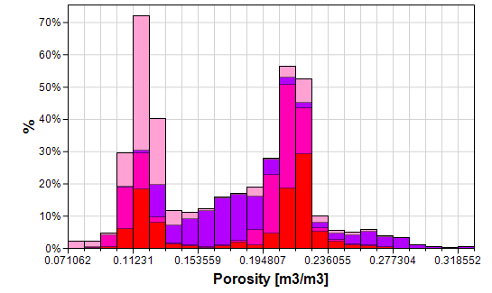 {width="5.677083333333333in" height="3.3854166666666665in"}
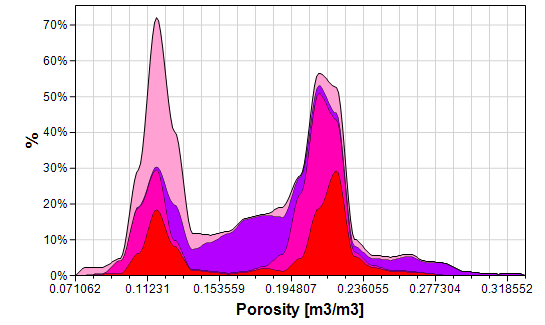 {width="5.677083333333333in" height="3.3854166666666665in"}]
[
{width="0.4166666666666667in" height="0.4166666666666667in"}]{.underline}[Toggle separate/stacked]{.underline}[
 {width="0.21875in" height="0.21875in"}]
[Toggle between showing bars/lines on top of each other
 {width="0.22916666666666666in" height="0.1875in"}, or side-by-side
  {width="0.19791666666666666in" height="0.1875in"}.]
[
{width="5.677083333333333in" height="3.3854166666666665in"}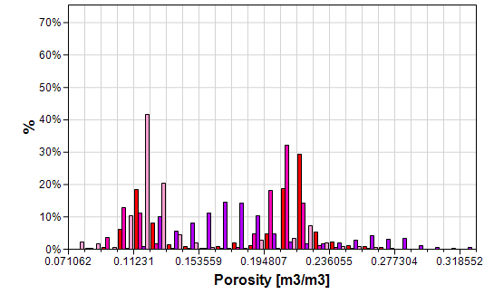 {width="5.677083333333333in" height="3.3854166666666665in"}]
[
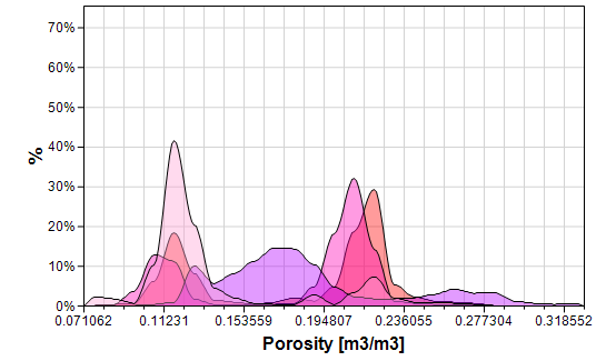 {width="5.677083333333333in" height="3.3854166666666665in"}]
[
{width="0.4166666666666667in" height="0.4166666666666667in"}]{.underline}[Toggle filled/empty]{.underline}[
 {width="0.23958333333333334in" height="0.21875in"}]
[Toggle between filled
 {width="0.21875in" height="0.1875in"} and empty
  {width="0.19791666666666666in" height="0.17708333333333334in"} bars/lines.]
[
{width="5.677083333333333in" height="3.3854166666666665in"}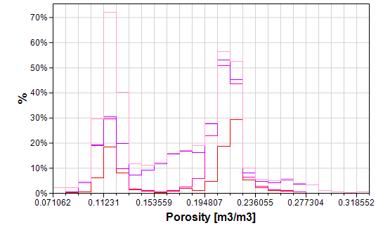 {width="5.677083333333333in" height="3.3854166666666665in"}]
[
{width="0.4166666666666667in" height="0.4166666666666667in"}]{.underline}[Toggle bar labels]{.underline}[
 {width="0.25in" height="0.2916666666666667in"}]
[Toggles bar label visibility. Bar labels are only displayed when bars are not stacked.]
[Note: Bar labels can only be displayed in the histogram window.]{.underline}
[
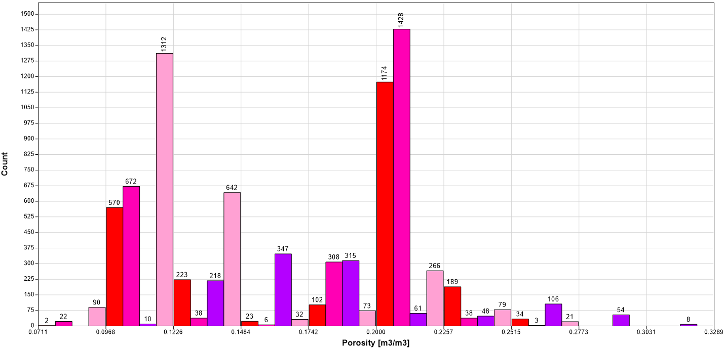 {width="5.677083333333333in" height="2.7604166666666665in"}
 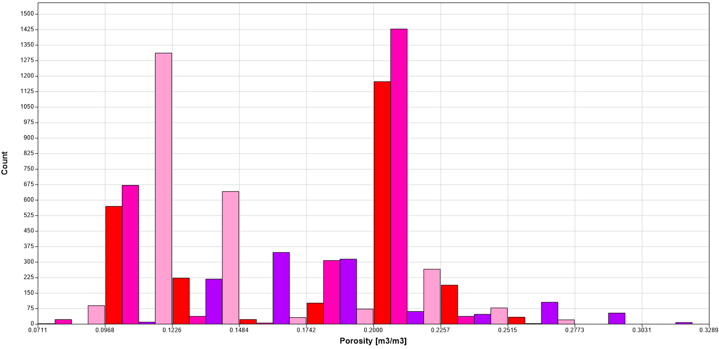 {width="5.677083333333333in" height="2.7604166666666665in"}]
[Multi-dimensions]{.underline}
[Controls which histograms are displayed.]
[
 {width="5.510416666666667in" height="0.4895833333333333in"}]
[
{width="0.4166666666666667in" height="0.4166666666666667in"}]{.underline}[Toggle multi-dimensions]{.underline}[
 {width="0.2916666666666667in" height="0.2916666666666667in"}]
[Toggles multi-dimension histograms]
[Note: Only available in histogram windows]{.underline}
[
{width="0.4166666666666667in" height="0.4166666666666667in"}]{.underline}[Show dimension data]{.underline}[
 {width="0.2916666666666667in" height="0.2916666666666667in"}]
[Controlling the displayed dimensions in Matrix plot and Parallel coordinates window is done using the ]{.underline}[Show dimension data]{.underline}[ drop down menu:]
[
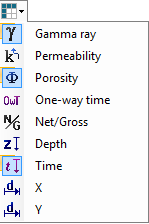 {width="1.5520833333333333in" height="2.3333333333333335in"}]
[Toggle the dimensions in the menu to decide what data to include in the plot:]
[
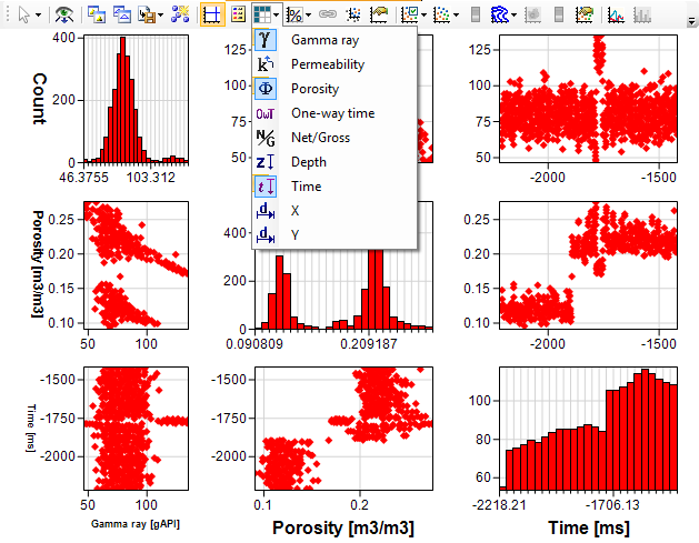 {width="6.197916666666667in" height="4.8125in"}]
[Bar chart]{.underline}
[
 {width="4.5625in" height="1.8541666666666667in"}]
[
{width="0.4166666666666667in" height="0.4166666666666667in"}]{.underline}[Bar chart]{.underline}[
 {width="0.25in" height="0.22916666666666666in"}]
[A dropdown menu allowing which discrete option should be used to bar chart. ]
[
 {width="1.4895833333333333in" height="1.0104166666666667in"}]
[See bar chart]{.underline} for more information.
[
{width="0.4166666666666667in" height="0.4166666666666667in"}]{.underline}[Bar chart statistics]{.underline}[
 {width="0.2708333333333333in" height="0.22916666666666666in"}]
[A dropdown menu allowing which statistic option is to be used to in the bar chart.]
[
 {width="1.3645833333333333in" height="2.0104166666666665in"}]
[
{width="0.4166666666666667in" height="0.4166666666666667in"}]{.underline}[Toggle view as datasets]{.underline}[
 {width="0.22916666666666666in" height="0.22916666666666666in"}]
[Toggle option allowing the bar chart to always be split into separate datasets. This is only enabled when datasets is not selected for both bar chart by and color by options. ]
[3D plot]{.underline}
[
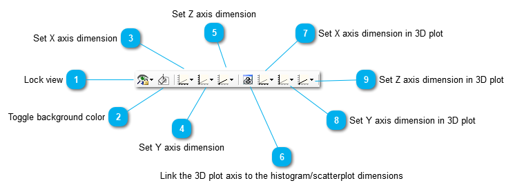 {width="6.197916666666667in" height="2.3020833333333335in"}]
[
{width="0.4166666666666667in" height="0.4166666666666667in"}]{.underline}[Lock view]{.underline}[
 {width="0.2916666666666667in" height="0.2916666666666667in"}]
[Select from this menu to lock the 3D plot to a chosen orientation.]
[
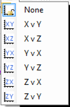 {width="1.4479166666666667in" height="2.2083333333333335in"}]
[Once locked the 3D plot cannot be rotated until the user selects the None option]
[
{width="0.4166666666666667in" height="0.4166666666666667in"}]{.underline}[Toggle background color]{.underline}[
 {width="0.2916666666666667in" height="0.2916666666666667in"}]
[Toggles the background color of the 3D plot between black and white]
[
{width="0.4166666666666667in" height="0.4166666666666667in"}]{.underline}[Set X axis dimension]{.underline}[
 {width="0.2916666666666667in" height="0.2916666666666667in"}]
[Sets the dimension to be displayed on the X axis. ]
[
{width="0.4166666666666667in" height="0.4166666666666667in"}]{.underline}[Set Y axis dimension]{.underline}[
 {width="0.2916666666666667in" height="0.2916666666666667in"}]
[Sets the dimension to be displayed on the Y axis. .]
[
{width="0.4166666666666667in" height="0.4166666666666667in"}]{.underline}[Set Z axis dimension]{.underline}[
 {width="0.2916666666666667in" height="0.2916666666666667in"}]
[Sets the dimension to be displayed on the Z axis. ]
[
{width="0.4166666666666667in" height="0.4166666666666667in"}]{.underline}[Link the 3D plot axis to the histogram/scatterplot dimensions]{.underline}[
 {width="0.2916666666666667in" height="0.2916666666666667in"}]
[Toggles linking the 3D plot axis dimensions with the axis dimensions used in the histograms/scatterplots.]
[
{width="0.4166666666666667in" height="0.4166666666666667in"}]{.underline}[Set X axis dimension in 3D plot]{.underline}[
 {width="0.2916666666666667in" height="0.2916666666666667in"}]
[Sets the dimension to be displayed on the X axis of the 3D plot when the plots are not linked]
[
{width="0.4166666666666667in" height="0.4166666666666667in"}]{.underline}[Set Y axis dimension in 3D plot]{.underline}[
 {width="0.2916666666666667in" height="0.2916666666666667in"}]
[Sets the dimension to be displayed on the Y axis of the 3D plot when the plots are not linked]
[
{width="0.4166666666666667in" height="0.4166666666666667in"}]{.underline}[Set Z axis dimension in 3D plot]{.underline}[
 {width="0.2916666666666667in" height="0.2916666666666667in"}]
[Sets the dimension to be displayed on the Z axis of the 3D plot when the plots are not linked]
[Time series]{.underline}
[
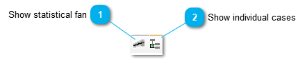 {width="4.604166666666667in" height="0.9270833333333334in"}]
[
{width="0.4166666666666667in" height="0.4166666666666667in"}]{.underline}[Show statistical fan]{.underline}[
 {width="0.25in" height="0.22916666666666666in"}]
[Used to quickly toggle whether summary result statistical fans are shown or not. . ]
[
{width="0.4166666666666667in" height="0.4166666666666667in"}]{.underline}[Show individual cases]{.underline}[
 {width="0.2708333333333333in" height="0.22916666666666666in"}]
[Used to quickly toggle whether individual summary results are shown or not. . ]
[Which individual summary results are shown can be controlled using this dialog:]
[
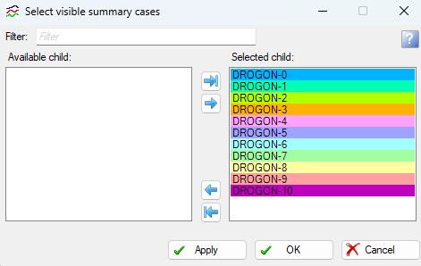 {width="4.90625in" height="3.1041666666666665in"}]
[which is accesed via the context menu on each dataset.]
[
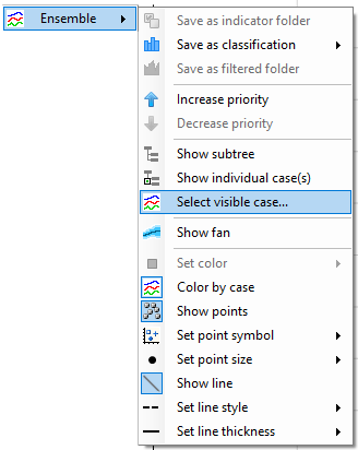 {width="3.4166666666666665in" height="4.291666666666667in"}]
[Show info on invalid plots]{.underline}
[
 {width="2.9895833333333335in" height="0.5in"}]
[
{width="0.4166666666666667in" height="0.4166666666666667in"}]{.underline}[Show info on invalid plots button]{.underline}[
 {width="0.2916666666666667in" height="0.2916666666666667in"}]
[If plot is highlighted with a yellow border, this button will be enabled in the toolbar. Click the button to open info dialog with information regarding the invalid plot(s).]
[Missing dimensions scenario]{.underline}
[The plot is invalid if there any of the data visible has missing dimensions. Dimensions can be added in the Data tab in the investigation settings. ]
[
{width="6.197916666666667in" height="4.302083333333333in"}][Dynamic equation cannot be defined scenario]{.underline}
[If there are no data visible in the plot the dynamic equation cannot be defined. Visualize some data in the window to validate the dynamic equation.]
[
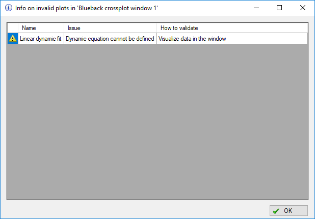 {width="6.197916666666667in" height="4.302083333333333in"}]
[Dynamic distribution equation cannot be defined scenario]{.underline}
[If the data that defines the distribution is no longer visible in the plot, the dynamic distribution equation cannot be defined. Visualize the data that defines the distribution in the window. ]
[
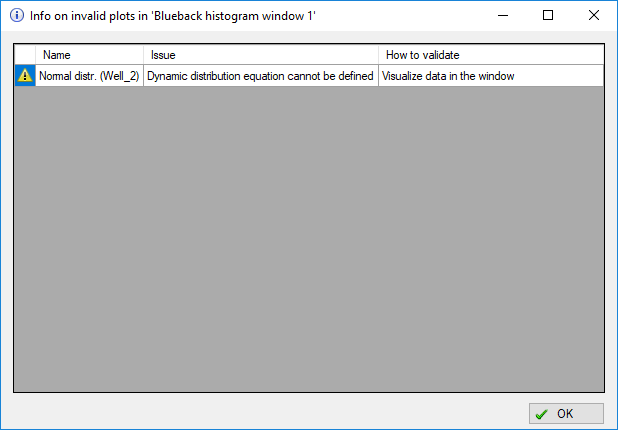 {width="6.197916666666667in" height="4.302083333333333in"}]
[Investigation settings dialog]{.underline}
[The settings dialog for the Blueback investigation contains tabs for controlling what data is displayed in the various plot windows and how it appears.]
[
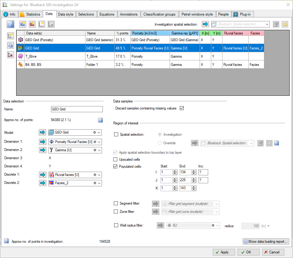 {width="6.197916666666667in" height="5.458333333333333in"}]
[It can be accessed by:]
[double-clicking on the Blueback investigation in the data tree]
[right-clicking in a Blueback plot and selecting ]{.underline}[Investigation Settings]{.underline}[ from the context menu]
[various buttons on the plot toolbars e.g. Data style settings
 {width="0.23958333333333334in" height="0.22916666666666666in"}, Equation settings
  {width="0.2604166666666667in" height="0.21875in"} etc.]
[
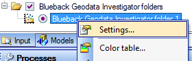 {width="2.9166666666666665in" height="0.9375in"}]
[Statistics tab]{.underline}
[The statistics tab shows some interesting characteristics about the investigation:]
[
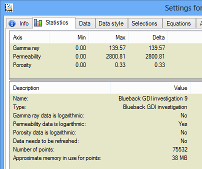 {width="4.208333333333333in" height="3.5208333333333335in"}]
[From the top:]
[Axis section - The data value range of the input data]
[Name - Name of the investigation]
[Type - Domain object type]
[Is logarithmic section - Is the dimension data logarithmic by default or not?]
[Data needs to be refreshed - Have the data points in the investigation been changed and a rebuild of the data engine is necessary?]
[Number of points - Number of points in the investigation]
[Approximate memory in use for points - Shows approximate memory usage for the points. ]{.underline}[N.B. The reported memory usage cannot be directly mapped to petrel.exe's memory usage in the Task Manager.]{.underline}
[Data tab]{.underline}
[See Data selection]{.underline} for information about the Data tab.
[Data style tab]{.underline}
[This tab allow the style of the data to be modified. Select one or more rows in the table and edit using the controls below.]
[
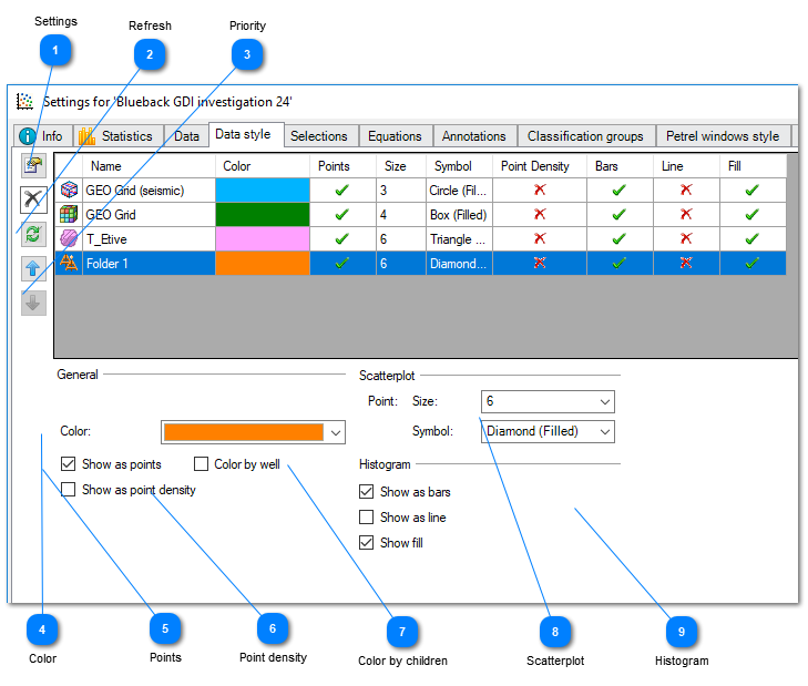 {width="6.197916666666667in" height="5.260416666666667in"}]
[
 {width="0.4166666666666667in" height="0.4166666666666667in"}]{.underline}[Settings]{.underline}
[
 {width="0.4166666666666667in" height="0.3541666666666667in"}]
[Opens the settings dialog for the selected row. This allows the statistics to be viewed.]
[
 {width="0.4166666666666667in" height="0.4166666666666667in"}]{.underline}[Refresh]{.underline}
[
 {width="0.4270833333333333in" height="0.3645833333333333in"}]
[Refresh the table.]
[
 {width="0.4166666666666667in" height="0.4166666666666667in"}]{.underline}[Priority]{.underline}
[
 {width="0.4270833333333333in" height="0.6770833333333334in"}]
[Blueback Investigator processes datasets in priority order - the highest item in the table has the highest priority. These buttons allow the order of datasets in the table to be altered by moving the selected row up or down. See dataset priority]{.underline} for more information
[
 {width="0.4166666666666667in" height="0.4166666666666667in"}]{.underline}[Color]{.underline}
[
 {width="3.1979166666666665in" height="0.2916666666666667in"}]
[Set the color for the selected data row(s).]
[
 {width="0.4166666666666667in" height="0.4166666666666667in"}]{.underline}[Points]{.underline}
[
 {width="1.3333333333333333in" height="0.2916666666666667in"}]
[Show the data as points.]
[
 {width="0.4166666666666667in" height="0.4166666666666667in"}]{.underline}[Point density]{.underline}
[
 {width="1.6875in" height="0.2916666666666667in"}]
[Show the data as point density. The visible area is gridded, and the number of points in each grid cell used to set the color. The number of bins used for the point density gridding is set from the Axis settings, either on the investigation scale ]{.underline}or window by window:
[
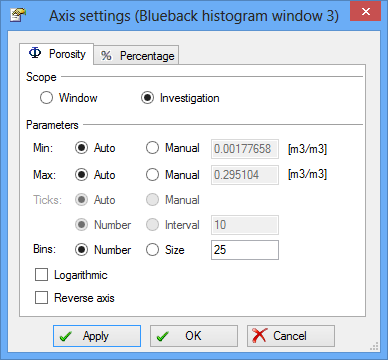 {width="4.041666666666667in" height="3.75in"}]
[The ]{.underline}[Bins]{.underline}[ setting controls the size of the point density rectangles. The point densities will stay the same size if a zoom is applied in the window.]
[
 {width="0.4166666666666667in" height="0.4166666666666667in"}]{.underline}[Color by children]{.underline}
[
 {width="1.4791666666666667in" height="0.2708333333333333in"}]
[For folders of wells and 2D seismic there is an extra option to allow the points to be colored by the child rather than the color set for the folder.]
[
 {width="0.4166666666666667in" height="0.4166666666666667in"}]{.underline}[Scatterplot]{.underline}
[
 {width="2.5729166666666665in" height="0.8958333333333334in"}]
[These controls enable the user to determine how the data is displayed on a scatterplot, allowing the size and symbol used to draw the points to be changed.]
[
 {width="0.4166666666666667in" height="0.4166666666666667in"}]{.underline}[Histogram]{.underline}
[
 {width="2.5520833333333335in" height="1.1458333333333333in"}]
[These controls determine how the data is displayed on a histogram - Use toggles to control the histogram data as (From left): ]
[bars]
[lines]
[lines/bars]
[
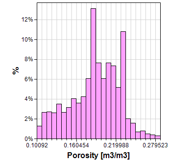 {width="3.6145833333333335in" height="3.46875in"}
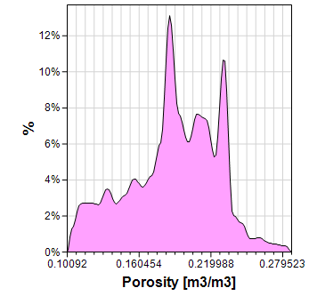 {width="3.6145833333333335in" height="3.46875in"}
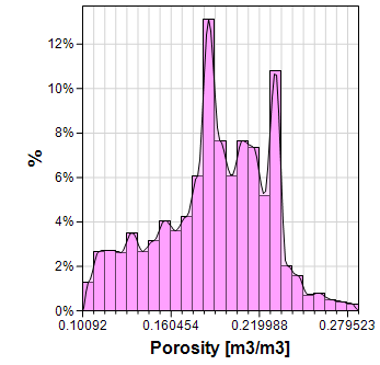 {width="3.6145833333333335in" height="3.46875in"}]
[Used in combination with the Show fill option you can display the above as (From left):]
[empty lines]
[empty bars]
[empty lines/bars]
[
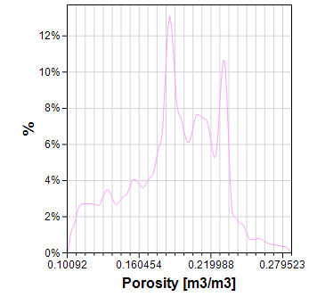 {width="3.6145833333333335in" height="3.46875in"}
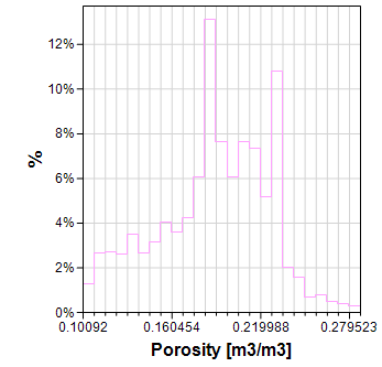 {width="3.6145833333333335in" height="3.46875in"}
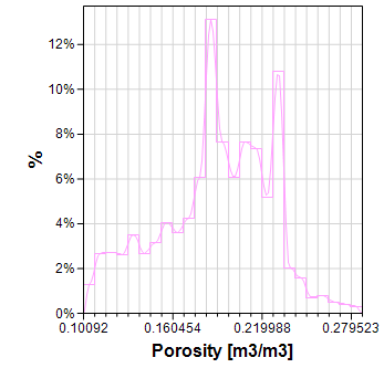 {width="3.6145833333333335in" height="3.46875in"}]
[Selections tab]{.underline}
[This tab allows the selections to be edited. Select one or more rows in the table and make changes using the controls below.]
[
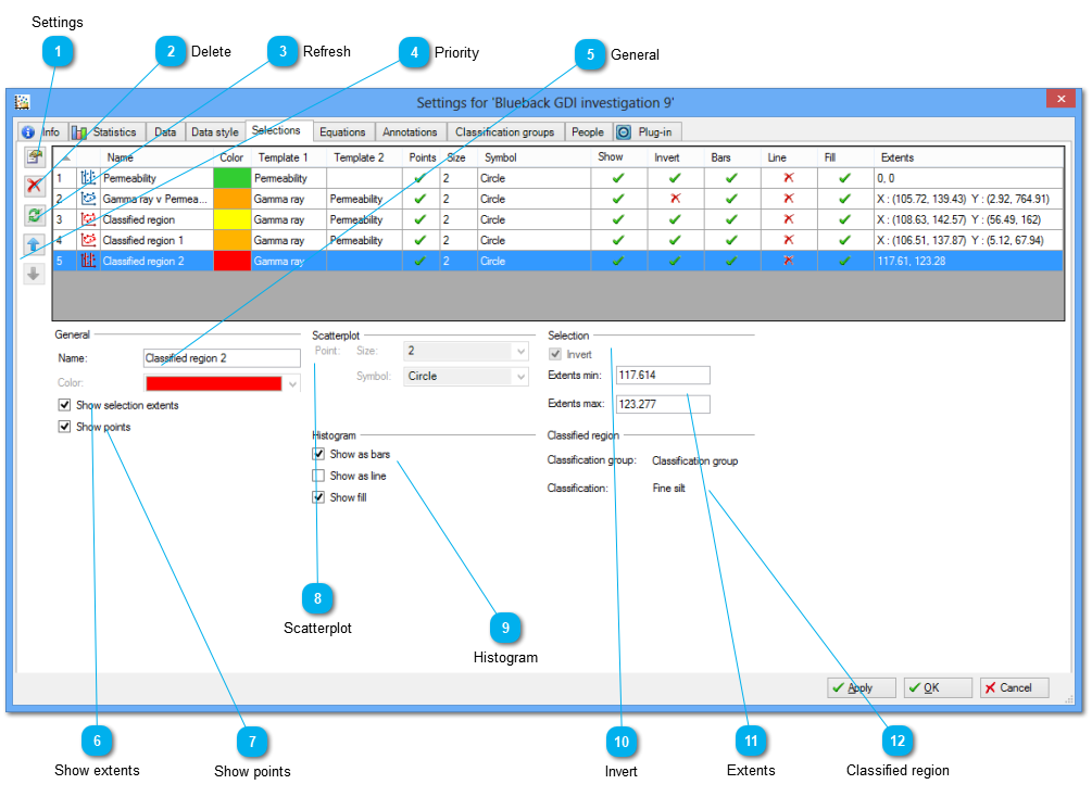 {width="6.197916666666667in" height="4.520833333333333in"}]
[
{width="0.4166666666666667in" height="0.4166666666666667in"}]{.underline}[Settings]{.underline}[
 {width="0.2916666666666667in" height="0.2916666666666667in"}]
[Opens the settings dialog for the selected row. This allows the statistics to be viewed.]
[
{width="0.4166666666666667in" height="0.4166666666666667in"}]{.underline}[Delete]{.underline}[
 {width="0.2916666666666667in" height="0.2916666666666667in"}]
[Removes the selected row.]
[
{width="0.4166666666666667in" height="0.4166666666666667in"}]{.underline}[Refresh]{.underline}[
 {width="0.2916666666666667in" height="0.2916666666666667in"}]
[Refresh the table.]
[
{width="0.4166666666666667in" height="0.4166666666666667in"}]{.underline}[Priority]{.underline}[
 {width="0.2916666666666667in" height="0.6354166666666666in"}]
[Selections are applied in order - the first item in the table has the highest priority. These buttons allow the order of selections in the table to be altered by moving the selected row up or down.]
[Filters always supercedes classifications. See Selection priority]{.underline} for more information
[
{width="0.4166666666666667in" height="0.4166666666666667in"}]{.underline}[General]{.underline}[
 {width="2.8229166666666665in" height="0.7916666666666666in"}]
[These controls allow the name and color of the selection to be changed.]
[
{width="0.4166666666666667in" height="0.4166666666666667in"}]{.underline}[Show extents]{.underline}[
 {width="1.4895833333333333in" height="0.2916666666666667in"}]
[This control allows the lines which specify the extents of the filter to be toggled on and off from the display.]
[
{width="0.4166666666666667in" height="0.4166666666666667in"}]{.underline}[Show points]{.underline}[
 {width="0.9479166666666666in" height="0.2916666666666667in"}]
[This control toggles whether or not the the points excluded by the filter are displayed.]
[
{width="0.4166666666666667in" height="0.4166666666666667in"}]{.underline}[Scatterplot]{.underline}[
 {width="2.5416666666666665in" height="0.7708333333333334in"}]
[These controls allow the size and symbol used for drawing excluded points to be changed.]
[
{width="0.4166666666666667in" height="0.4166666666666667in"}]{.underline}[Histogram]{.underline}[
 {width="2.5625in" height="0.9270833333333334in"}]
[If 'Show points' is selected, then the excluded points are displayed in the histogram window as a separate dataset. These controls allow how the data is drawn in the histogram to be changed - see the Appearance tab]{.underline} help page for details.
[
{width="0.4166666666666667in" height="0.4166666666666667in"}]{.underline}[Invert]{.underline}[
 {width="0.65625in" height="0.2916666666666667in"}]
[Filters by default are inclusive, that is points inside the filter are considered as 'selected'. This control allow the filters to be inverted, so that the filter becomes exclusive.]
[Note - Only Blueback filters can be inverted.]
[
{width="0.4166666666666667in" height="0.4166666666666667in"}]{.underline}[Extents]{.underline}[
 {width="1.9166666666666667in" height="0.5833333333333334in"}]
[For vertical and horizontal selections, the extents of the filter can be edited using these controls.]
[
{width="0.4166666666666667in" height="0.4166666666666667in"}]{.underline}[Classified region]{.underline}[
 {width="2.3645833333333335in" height="0.875in"}]
[Displays info about what group and classification that has been set for the classification selections.]
[Equations tab]{.underline}
[This tab allows the settings of equations to be changed. Select one or more rows in the table and use the controls below to make changes.]
[
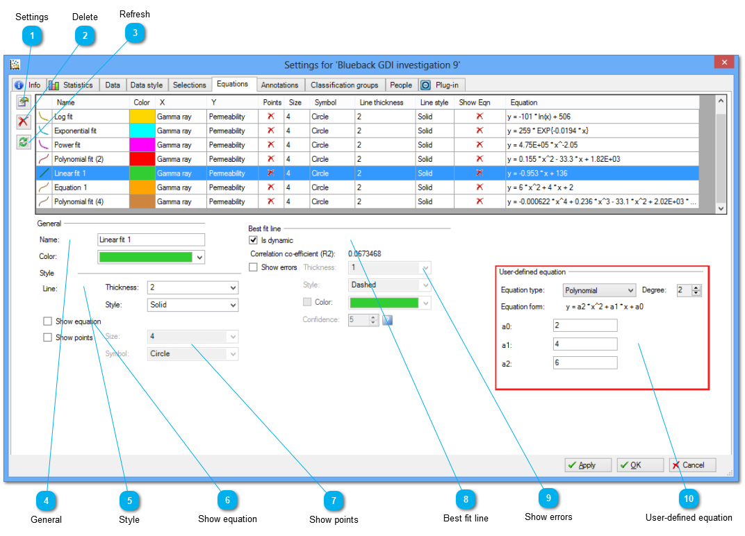 {width="6.197916666666667in" height="4.458333333333333in"}]
[
{width="0.4166666666666667in" height="0.4166666666666667in"}]{.underline}[Settings]{.underline}[
 {width="0.2916666666666667in" height="0.2916666666666667in"}]
[Open the settings dialogs for the selected equations.]
[
{width="0.4166666666666667in" height="0.4166666666666667in"}]{.underline}[Delete]{.underline}[
 {width="0.2916666666666667in" height="0.2916666666666667in"}]
[Delete the selected equations.]
[
{width="0.4166666666666667in" height="0.4166666666666667in"}]{.underline}[Refresh]{.underline}[
{width="0.2916666666666667in" height="0.2916666666666667in"}][Refresh the table.]
[
{width="0.4166666666666667in" height="0.4166666666666667in"}]{.underline}[General]{.underline}[
 {width="2.84375in" height="0.8125in"}]
[These controls allow the name of the equation and the color to be changed.]
[
{width="0.4166666666666667in" height="0.4166666666666667in"}]{.underline}[Style]{.underline}[
 {width="3.3645833333333335in" height="0.7708333333333334in"}]
[These controls change the thickness and style of the line as drawn in the plot windows.]
[
{width="0.4166666666666667in" height="0.4166666666666667in"}]{.underline}[Show equation]{.underline}[
 {width="1.1145833333333333in" height="0.2604166666666667in"}]
[Sets whether or not the equation of the line is displayed adjacent to the line on the plot.]
[
{width="0.4166666666666667in" height="0.4166666666666667in"}]{.underline}[Show points]{.underline}[
 {width="3.2916666666666665in" height="0.5729166666666666in"}]
[Controls whether the points used to plot the line in the window will be drawn. If selected, the size and symbol of the points can be changed.]
[
{width="0.4166666666666667in" height="0.4166666666666667in"}]{.underline}[Best fit line]{.underline}[
 {width="3.2395833333333335in" height="0.6041666666666666in"}]
[The ]{.underline}[Is dynamic]{.underline}[ check box controls if an equation is dynamic or not.]
[The R2 correlation coefficient displays the R2 for the selected equation.]
[R2 can in some cases become negative]{.underline} (Article from http://stats.stackexchange.com/questions/12900/when-is-r-squared-negative).
[See this article for information on the R2 implementation: ]
[Weisstein, Eric W. "Correlation Coefficient." From MathWorld--A Wolfram Web Resource. ]{.underline}
[
{width="0.4166666666666667in" height="0.4166666666666667in"}]{.underline}[Show errors]{.underline}[
 {width="3.1666666666666665in" height="1.1666666666666667in"}]
[For linear, log, exponential and power law fit lines, the errors can be displayed. The thickness, style and color of the line can all be changed.]
[The lines drawn on the plot correspond to the degree of confidence as set by the confidence control.]
[
{width="0.4166666666666667in" height="0.4166666666666667in"}]{.underline}[User-defined equation]{.underline}[
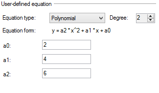 {width="3.3854166666666665in" height="1.96875in"}]
[If a user-defined equation is selected then this set of controls will be displayed. The equation type can be modified using the drop menu. For polynomial equations, the polynomial degree can be set. The equation coefficients can be edited to modify the line. ]
[Annotations tab]{.underline}
[This tabs allows annotation text and style to be updated. Select one or more rows in the table and make the changes using the controls below.]
[
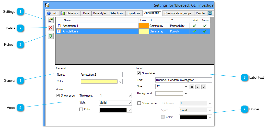 {width="6.197916666666667in" height="2.9583333333333335in"}]
[
{width="0.4166666666666667in" height="0.4166666666666667in"}]{.underline}[Settings]{.underline}[
 {width="0.2916666666666667in" height="0.2916666666666667in"}]
[Open the settings dialogs for the selected annotations.]
[
{width="0.4166666666666667in" height="0.4166666666666667in"}]{.underline}[Delete]{.underline}[
{width="0.2916666666666667in" height="0.2916666666666667in"}][Delete the selected annotations.]
[
{width="0.4166666666666667in" height="0.4166666666666667in"}]{.underline}[Refresh]{.underline}[
 {width="0.2916666666666667in" height="0.2916666666666667in"}]
[Refresh the table.]
[
{width="0.4166666666666667in" height="0.4166666666666667in"}]{.underline}[General]{.underline}[
 {width="2.8229166666666665in" height="0.7916666666666666in"}]
[Set the name of this annotation (note: not the annotation text) and the color.]
[
{width="0.4166666666666667in" height="0.4166666666666667in"}]{.underline}[Arrow]{.underline}[
 {width="3.25in" height="1.0625in"}]
[Optionally display an arrow from the annotation to a point of interest. Set the thickness, style and color of the arrow here.]
[The arrow head will initially point to the same position on the plot where the text was added, so it will be hidden. Click on the annotation in the plot window and drag it out of the way to see the arrow. The arrow head can then also be dragged around the plot window.]
[
{width="0.4166666666666667in" height="0.4166666666666667in"}]{.underline}[Label text]{.underline}[
 {width="3.2291666666666665in" height="1.2916666666666667in"}]
[Set the text for the label, and the font size, style and background color.]
[
{width="0.4166666666666667in" height="0.4166666666666667in"}]{.underline}[Border]{.underline}[
 {width="3.1875in" height="0.9270833333333334in"}]
[Optionally display a border around the text, setting the thickness, style and color.]
[Classification groups tab]{.underline}
[Create and edit Classification groups to be used in classification workflow. Edit multiple groups by highlighting multiple rows in the table.]
[A classification group is similar to a discrete Petrel template, but with the difference that it has two built in discrete codes; Filtered and Unclassified. Once created, the group is linked to an external physical template with the Name set under Template.]
[
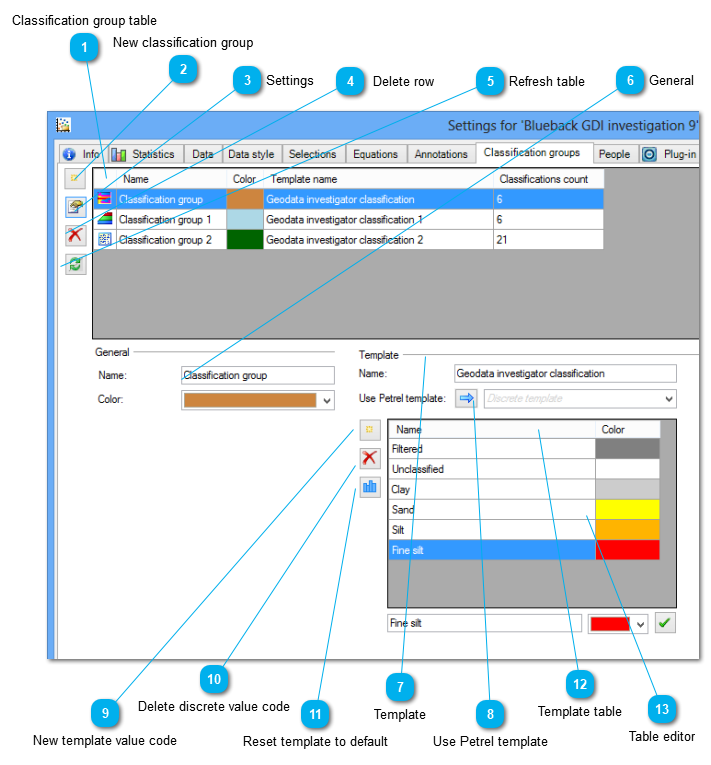 {width="6.197916666666667in" height="6.666666666666667in"}]
[
{width="0.4166666666666667in" height="0.4166666666666667in"}]{.underline}[Classification group table]{.underline}[
 {width="6.010416666666667in" height="1.1354166666666667in"}]
[Table showing all the available Classification groups belonging to an investigation. ]
[
{width="0.4166666666666667in" height="0.4166666666666667in"}]{.underline}[New classification group]{.underline}[
 {width="0.34375in" height="0.3229166666666667in"}]
[Create new classification row in the table. The new template will be based on the Petrel General discrete template.]
[
{width="0.4166666666666667in" height="0.4166666666666667in"}]{.underline}[Settings]{.underline}[
 {width="0.3645833333333333in" height="0.3645833333333333in"}]
[Show settings for the selected row.]
[
{width="0.4166666666666667in" height="0.4166666666666667in"}]{.underline}[ Delete row]{.underline}[
 {width="0.3645833333333333in" height="0.3645833333333333in"}]
[Delete the selected classification group(s)]
[
{width="0.4166666666666667in" height="0.4166666666666667in"}]{.underline}[Refresh table]{.underline}[
 {width="0.3645833333333333in" height="0.3645833333333333in"}]
[Refreshes the table.]
[
{width="0.4166666666666667in" height="0.4166666666666667in"}]{.underline}[General]{.underline}[
 {width="2.875in" height="0.8854166666666666in"}]
[Change name and color of the classification group.]
[
{width="0.4166666666666667in" height="0.4166666666666667in"}]{.underline}[Template]{.underline}[
 {width="3.6458333333333335in" height="0.4375in"}]
[Change the name of the new template to be made.]
[
{width="0.4166666666666667in" height="0.4166666666666667in"}]{.underline}[Use Petrel template]{.underline}[
 {width="3.7083333333333335in" height="0.3333333333333333in"}]
[Copies the template value codes into the group. If done multiple times, the codes are added to the list.]
[
{width="0.4166666666666667in" height="0.4166666666666667in"}]{.underline}[New template value code]{.underline}[
 {width="0.2916666666666667in" height="0.2916666666666667in"}]
[Insert new template value code.]
[
{width="0.4166666666666667in" height="0.4166666666666667in"}]{.underline}[Delete discrete value code]{.underline}[
{width="0.3645833333333333in" height="0.3645833333333333in"}][Deletes the selected value code row]
[
{width="0.4166666666666667in" height="0.4166666666666667in"}]{.underline}[Reset template to default]{.underline}[
 {width="0.3645833333333333in" height="0.3645833333333333in"}]
[Resets table to display the Petrel General discrete template with the added Filtered and Unclassified filters.]
[
{width="0.4166666666666667in" height="0.4166666666666667in"}]{.underline}[Template table]{.underline}[
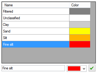 {width="3.375in" height="2.53125in"}]
[Template editor. Use Table editor]{.underline} to edit the active row.
[
{width="0.4166666666666667in" height="0.4166666666666667in"}]{.underline}[Table editor]{.underline}[
 {width="3.4166666666666665in" height="0.3229166666666667in"}]
[Edit the value code name and color. Use the
 {width="0.2708333333333333in" height="0.28125in"} button to apply the changes locally to the table.]
[Petrel window style tab]{.underline}
[The Petrel window style tab allows the user to control how the investigation is displayed in Petrel windows.]
[This tab will be enabled when a Petrel window is active and the investigation is toggled for display.]
[Changes made on this dialog immediately update the investigation in the Petrel window.]
[
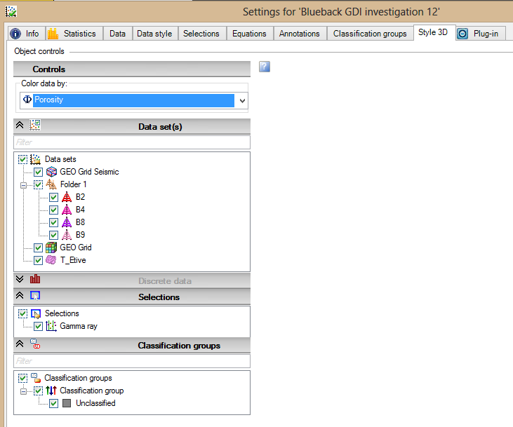 {width="6.197916666666667in" height="5.15625in"}]
[Tools]{.underline}
[Blueback Investigator provides tools which can be used to speed up common data visualization and analysis tasks. ]
[These tools are based on the Blueback Toolbox or Marina style of tool as used in other Blueback products.]
[Quick start histogram tool]{.underline}
[Note: This tool has been deprecated as it was causing confusion (please contact ]{.underline}[support]{.underline} if access is still required)
[This tool can be used to create and view histograms based on various input data types. The tool provides the option to create a new Blueback investigation from the input data, as well as the option to show a new histogram window for that investigation and to provide a name for that investigation.]
[At least one of the selected input data type objects must be provided along with a continuous dimension for the histogram to display data and for the tool to produce output.]
[An area of interest can be defined for certain input data types. If an input data type that supports this is selected, controls for specifying the region of interest will be presented in the 'egion of Interest'box.]
[Quick start histogram tool dialog (overview)]{.underline}
[
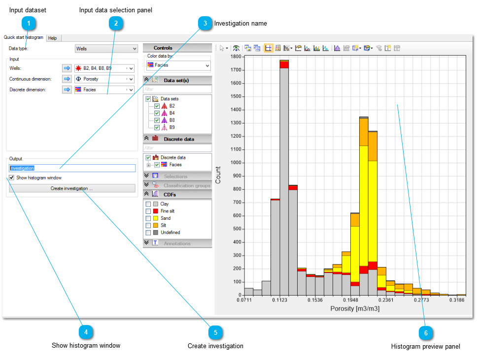 {width="6.197916666666667in" height="4.65625in"}]
[
{width="0.4166666666666667in" height="0.4166666666666667in"}]{.underline}[Input dataset ]{.underline}[
 {width="3.5416666666666665in" height="0.2916666666666667in"}]
[Select the input dataset type to plot and create investigations from. Updates the displayed Input data selection panel]{.underline}.
[
{width="0.4166666666666667in" height="0.4166666666666667in"}]{.underline}[Input data selection panel]{.underline}[
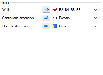 {width="3.5208333333333335in" height="2.5729166666666665in"}]
[Select source dataset objects, continuous and discrete dimensions and specify regions of interest for plotting and creating investigations. See individual help files for further details on each panel:]
[
{width="0.4166666666666667in" height="0.4166666666666667in"}]{.underline}[Investigation name]{.underline}[
 {width="3.4479166666666665in" height="0.3229166666666667in"}]
[Define the name of this investigation]
[
{width="0.4166666666666667in" height="0.4166666666666667in"}]{.underline}[Show histogram window]{.underline}[
 {width="1.59375in" height="0.2916666666666667in"}]
[If selected, displays the supplied input dataset and related parameters in a new Blueback Investigator Histogram window when create investigation is clicked]
[
{width="0.4166666666666667in" height="0.4166666666666667in"}]{.underline}[Create investigation]{.underline}[
 {width="3.4375in" height="0.2916666666666667in"}]
[The creates a new Blueback investigation using the supplied input dataset and related parameters.]
[
{width="0.4166666666666667in" height="0.4166666666666667in"}]{.underline}[Histogram preview panel]{.underline}[
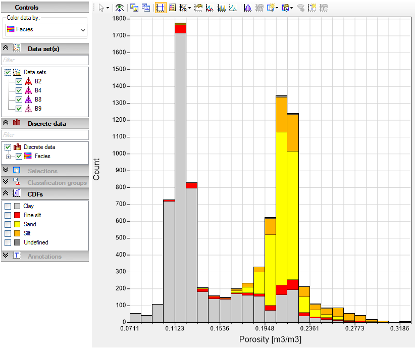 {width="6.197916666666667in" height="5.1875in"}]
[Provides a histogram plot of the supplied input dataset and related parameters.]
[Well data selection panel dialog]{.underline}
[
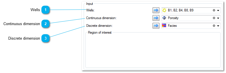 {width="6.197916666666667in" height="2.0in"}]
[This panel can be displayed by selecting the Input dataset]{.underline}.
[
{width="0.4166666666666667in" height="0.4166666666666667in"}]{.underline}[Wells]{.underline}[
 {width="4.9375in" height="0.2916666666666667in"}]
[Select one or more wells for use as an input dataset.]
[
{width="0.4166666666666667in" height="0.4166666666666667in"}]{.underline}[Continuous dimension]{.underline}[
 {width="4.979166666666667in" height="0.2916666666666667in"}]
[Select a single global well log for use as a continuous dimension.]
[
{width="0.4166666666666667in" height="0.4166666666666667in"}]{.underline}[Discrete dimension]{.underline}[
 {width="4.96875in" height="0.2916666666666667in"}]
[Select a single discrete global well log for use as a discrete dimension.]
[Seismic data selection panel dialog]{.underline}
[
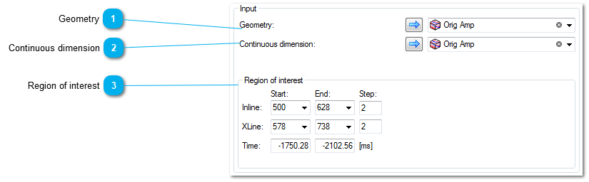 {width="6.197916666666667in" height="1.9166666666666667in"}]
[This panel can be displayed by selecting the Input dataset]{.underline}.
[
{width="0.4166666666666667in" height="0.4166666666666667in"}]{.underline}[Geometry]{.underline}[
 {width="4.947916666666667in" height="0.2916666666666667in"}]
[Select a single seismic cube as a geometry for use as an input dataset.]
[
{width="0.4166666666666667in" height="0.4166666666666667in"}]{.underline}[Continuous dimension]{.underline}[
 {width="4.979166666666667in" height="0.2916666666666667in"}]
[Select a single seismic cube for use as a continuous dimension.]
[
{width="0.4166666666666667in" height="0.4166666666666667in"}]{.underline}[Region of interest]{.underline}[
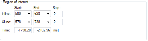 {width="4.96875in" height="1.3854166666666667in"}]
[Allows specification of a region of interest for the selected seismic cube geometry. The start, end and step values for Inline and Crossline can be specified, as well as a time range. Note that the default values for the step controls are set to limit the number of data points to less than 100000 when a geometry is selected. This is for performance reasons. It can be overridden by simply selecting a smaller step, at the cost of greater processing time.]
[Model data selection panel dialog]{.underline}
[
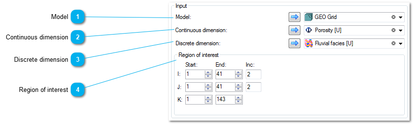 {width="6.197916666666667in" height="1.875in"}]
[This panel can be displayed by selecting the Input dataset]{.underline}.
[
{width="0.4166666666666667in" height="0.4166666666666667in"}]{.underline}[Model]{.underline}[
 {width="5.041666666666667in" height="0.2916666666666667in"}]
[Select a model for use as an input dataset.]
[
{width="0.4166666666666667in" height="0.4166666666666667in"}]{.underline}[Continuous dimension]{.underline}[
 {width="4.989583333333333in" height="0.2916666666666667in"}]
[Select a model property for use as a continuous dimension.]
[
{width="0.4166666666666667in" height="0.4166666666666667in"}]{.underline}[Discrete dimension]{.underline}[
 {width="5.020833333333333in" height="0.2916666666666667in"}]
[Select a model discrete property for use as a discrete dimension.]
[
{width="0.4166666666666667in" height="0.4166666666666667in"}]{.underline}[Region of interest]{.underline}[
 {width="4.979166666666667in" height="1.4166666666666667in"}]
[Allows specification of a region of interest for the selected model. The start and end values for the I, J and K dimensions can be specified. In addition, the increment values for the I and J dimensions can be specified. Note that the default values for the increment controls are set to limit the number of data points to less than 100000 when a model is selected. This is for performance reasons. It can be overridden by simply selecting a smaller increment, at the cost of greater processing time.]
[Quick start crossplot tool]{.underline}
[Note: This tool has been deprecated as it was causing confusion (please contact ]{.underline}[support]{.underline} if access is still required)
[This tool can be used to create and view crossplots based on various input data types. The tool provides the option to create a new Blueback investigation from the input data, as well as the option to show a new crossplot window for that investigation and to provide a name for that investigation.]
[At least one of the selected input data type objects must be provided along with two continuous dimensions for the crossplot to display data and for the tool to produce output.]
[An area of interest can be defined for certain input data types. If an input data type that supports this is selected, controls for specifying the region of interest will be presented in the 'egion of Interest'box.]
[Quick start crossplot tool dialog (overview)]{.underline}
[
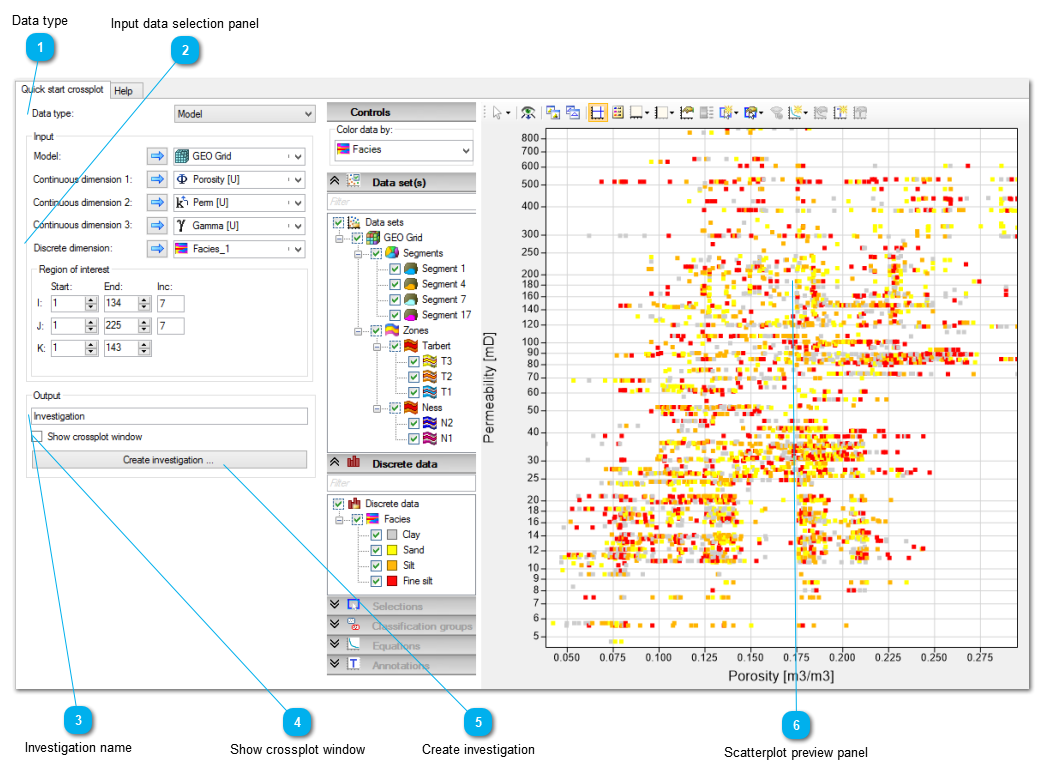 {width="6.197916666666667in" height="4.625in"}]
[
{width="0.4166666666666667in" height="0.4166666666666667in"}]{.underline}[Data type]{.underline}[
 {width="3.6875in" height="0.3333333333333333in"}]
[Select the input dataset type to plot and create investigations from. Updates the displayed Input data selection panel]{.underline}.
[
{width="0.4166666666666667in" height="0.4166666666666667in"}]{.underline}[Input data selection panel]{.underline}[
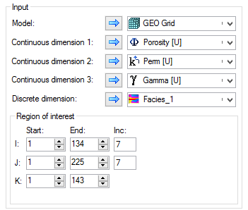 {width="3.65625in" height="3.1041666666666665in"}]
[Select source dataset objects, continuous and discrete dimensions and specify regions of interest for plotting and creating investigations. See individual help files for further details on each panel:]
[
{width="0.4166666666666667in" height="0.4166666666666667in"}]{.underline}[Investigation name]{.underline}[
 {width="3.4895833333333335in" height="0.2916666666666667in"}]
[Define the name of this investigation]
[
{width="0.4166666666666667in" height="0.4166666666666667in"}]{.underline}[Show crossplot window]{.underline}[
 {width="1.6145833333333333in" height="0.2916666666666667in"}]
[If selected, displays the supplied input dataset and related parameters in a new Blueback Blueback Investigator Crossplot window when create investigation is clicked]
[
{width="0.4166666666666667in" height="0.4166666666666667in"}]{.underline}[Create investigation]{.underline}[
 {width="3.4895833333333335in" height="0.2916666666666667in"}]
[The creates a new Blueback investigation using the supplied input dataset and related parameters.]
[
{width="0.4166666666666667in" height="0.4166666666666667in"}]{.underline}[Scatterplot preview panel]{.underline}[
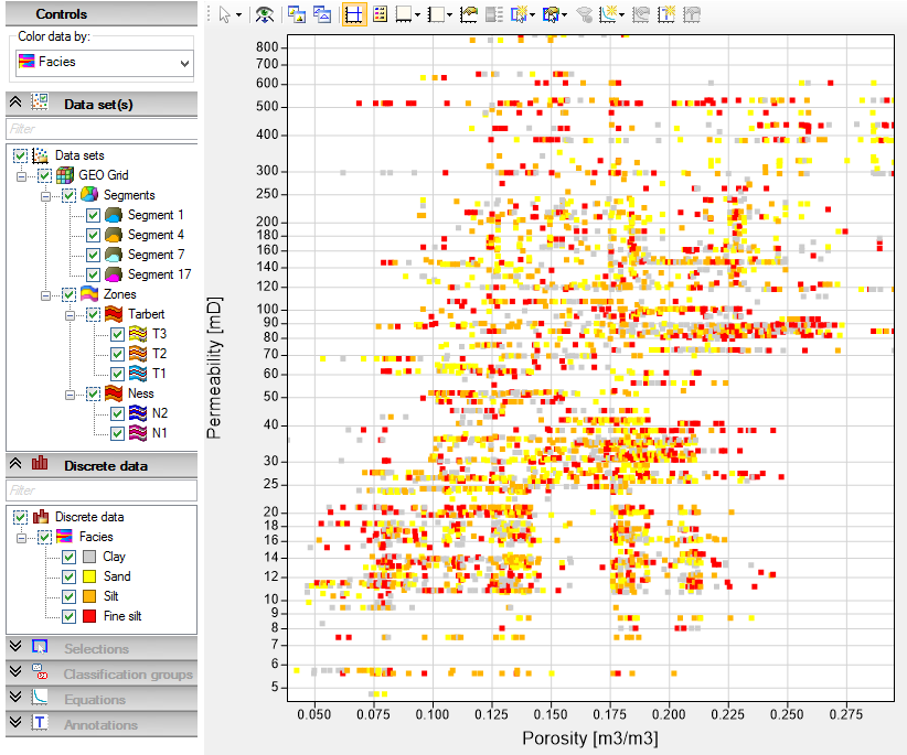 {width="6.197916666666667in" height="5.15625in"}]
[Provides a scatterplot of the supplied input dataset and related parameters.]
[Well data selection panel dialog]{.underline}
[
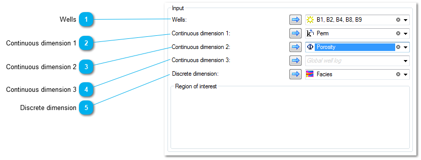 {width="6.197916666666667in" height="2.3541666666666665in"}]
[This panel can be displayed by selecting the appropriate Data type]{.underline}.
[
{width="0.4166666666666667in" height="0.4166666666666667in"}]{.underline}[Wells]{.underline}[
 {width="4.958333333333333in" height="0.2916666666666667in"}]
[Select one or more wells for use as an input dataset.]
[
{width="0.4166666666666667in" height="0.4166666666666667in"}]{.underline}[Continuous dimension 1]{.underline}[
 {width="5.0in" height="0.2916666666666667in"}]
[Select a single global well log for use as a continuous dimension.]
[
{width="0.4166666666666667in" height="0.4166666666666667in"}]{.underline}[Continuous dimension 2]{.underline}[
 {width="4.958333333333333in" height="0.2916666666666667in"}]
[Select a single global well log for use as a continuous dimension.]
[
{width="0.4166666666666667in" height="0.4166666666666667in"}]{.underline}[Continuous dimension 3]{.underline}[
 {width="4.958333333333333in" height="0.2916666666666667in"}]
[Select a single global well log for use as a continuous dimension. If selected, this dimension is used to color the scatterplot points.]
[
{width="0.4166666666666667in" height="0.4166666666666667in"}]{.underline}[Discrete dimension]{.underline}[
 {width="4.96875in" height="0.2916666666666667in"}]
[Select a single discrete global well log for use as a discrete dimension. If selected, this dimension is used to color the scatterplot points.]
[Seismic data selection panel dialog]{.underline}
[
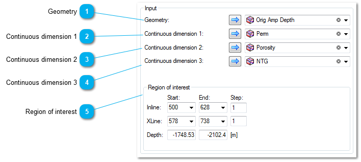 {width="6.197916666666667in" height="2.7708333333333335in"}]
[This panel can be displayed by selecting the appropriate Data type]{.underline}.
[
{width="0.4166666666666667in" height="0.4166666666666667in"}]{.underline}[Geometry]{.underline}[
 {width="4.302083333333333in" height="0.2916666666666667in"}]
[Select a single seismic cube as a geometry for use as an input dataset.]
[
{width="0.4166666666666667in" height="0.4166666666666667in"}]{.underline}[Continuous dimension 1]{.underline}[
 {width="4.291666666666667in" height="0.2916666666666667in"}]
[Select a single seismic cube for use as a continuous dimension.]
[
{width="0.4166666666666667in" height="0.4166666666666667in"}]{.underline}[Continuous dimension 2]{.underline}[
 {width="4.354166666666667in" height="0.2916666666666667in"}]
[Select a single seismic cube for use as a continuous dimension.]
[
{width="0.4166666666666667in" height="0.4166666666666667in"}]{.underline}[Continuous dimension 3]{.underline}[
 {width="4.3125in" height="0.2916666666666667in"}]
[Select a single seismic cube for use as a continuous dimension. If selected, this dimension is used to color the scatterplot points.]
[
{width="0.4166666666666667in" height="0.4166666666666667in"}]{.underline}[Region of interest]{.underline}[
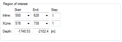 {width="4.302083333333333in" height="1.4791666666666667in"}]
[Allows specification of a region of interest for the selected seismic cube geometry. The start, end and step values for Inline and Crossline can be specified, as well as a time range. Note that the default values for the step controls are set to limit the number of data points to less than 100000 when a geometry is selected. This is for performance reasons. It can be overridden by simply selecting a smaller step, at the cost of greater processing time.]
[Model data selection panel dialog]{.underline}
[
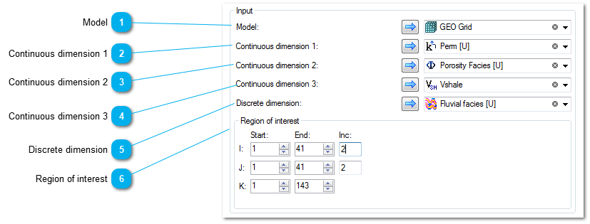 {width="6.197916666666667in" height="2.3541666666666665in"}]
[This panel can be displayed by selecting the appropriate Data type]{.underline}.
[
{width="0.4166666666666667in" height="0.4166666666666667in"}]{.underline}[Model]{.underline}[
 {width="5.052083333333333in" height="0.2916666666666667in"}]
[Select a model for use as an input dataset.]
[
{width="0.4166666666666667in" height="0.4166666666666667in"}]{.underline}[Continuous dimension 1]{.underline}[
 {width="5.010416666666667in" height="0.2916666666666667in"}]
[Select a model property for use as a continuous dimension.]
[
{width="0.4166666666666667in" height="0.4166666666666667in"}]{.underline}[Continuous dimension 2]{.underline}[
 {width="4.947916666666667in" height="0.2916666666666667in"}]
[Select a model property for use as a continuous dimension.]
[
{width="0.4166666666666667in" height="0.4166666666666667in"}]{.underline}[Continuous dimension 3]{.underline}[
 {width="4.947916666666667in" height="0.2916666666666667in"}]
[Select a model property for use as a continuous dimension. If selected, this dimension is used to color the scatterplot points.]
[
{width="0.4166666666666667in" height="0.4166666666666667in"}]{.underline}[Discrete dimension]{.underline}[
 {width="4.947916666666667in" height="0.2916666666666667in"}]
[Select a model discrete property for use as a discrete dimension.]
[
{width="0.4166666666666667in" height="0.4166666666666667in"}]{.underline}[Region of interest]{.underline}[
 {width="5.010416666666667in" height="1.40625in"}]
[Allows specification of a region of interest for the selected model. The start and end values for the I, J and K dimensions can be specified. In addition, the increment values for the I and J dimensions can be specified. Note that the default values for the increment controls are set to limit the number of data points to less than 100000 when a model is selected. This is for performance reasons. It can be overridden by simply selecting a smaller increment, at the cost of greater processing time.]
[Equation transformer tool]{.underline}
[This tool can be used to create new Petrel domain objects using Blueback Investigator equations.]
[The tool can apply any equation defined in the investigation. The available equations in an investigation also includes user defined classifications (ie. classifications which use digitized classified regions to define the different areas within a plot)]
[Equation transformer tool dialog]{.underline}
[
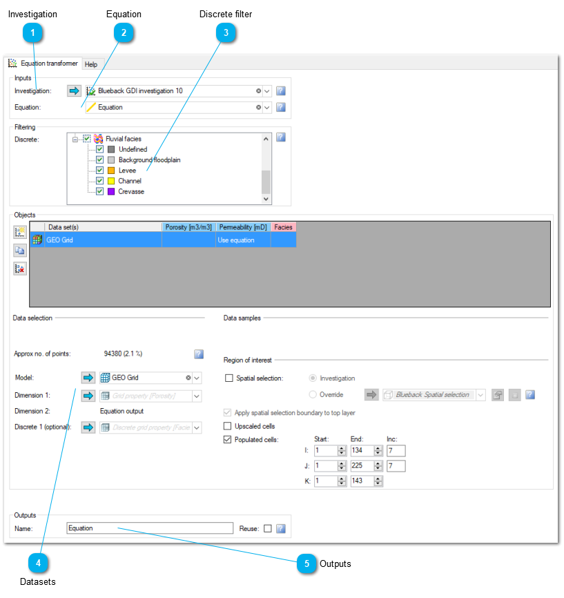 {width="6.197916666666667in" height="6.5625in"}]
[
{width="0.4166666666666667in" height="0.4166666666666667in"}]{.underline}[Investigation]{.underline}[
 {width="4.6875in" height="0.3333333333333333in"}]
[Select the investigation containing the equation to use. Only investigations containing equations will be shown.]
[
{width="0.4166666666666667in" height="0.4166666666666667in"}]{.underline}[Equation]{.underline}[
 {width="4.666666666666667in" height="0.2916666666666667in"}]
[Select the equation to be used to transform. This list will include both equations and user defined classifications.]
[
{width="0.4166666666666667in" height="0.4166666666666667in"}]{.underline}[Discrete filter]{.underline}[
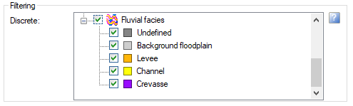 {width="5.15625in" height="1.5520833333333333in"}]
[Define the name of this investigation]
[
{width="0.4166666666666667in" height="0.4166666666666667in"}]{.underline}[Datasets]{.underline}[
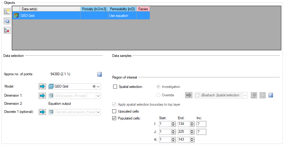 {width="6.197916666666667in" height="3.1979166666666665in"}]
[Use this table to define the datasets to be processed. Select the required Petrel domain objects and specify a region of interest if necessary.]
[
{width="0.4166666666666667in" height="0.4166666666666667in"}]{.underline}[Outputs]{.underline}[
 {width="4.958333333333333in" height="0.2916666666666667in"}]
[Use this to define the label to be used to identify the output Petrel domain objects. ]
[Optionally the output can be reused. This allows different equations to be used to ]{.underline}[build]{.underline}[ the output data, eg use a different equation in sands and shales.]
[Data reshaper tool]{.underline}
[The data reshaper tool can be used to reshape ]{.underline}[well log]{.underline}[ data to fit a target distribution or a specific range.]
[The reshaping can be done in three different ways:]
[Fit to a distribution. The data is shifted, squeezed or stretched so that the resulting data matches a given distribution. The target distribution must be either]
a. [A ]{.underline}[normal distribution]{.underline}[, in which case the resulting data will have a mean and standard deviation that matches the target distribution.]
b. [A ]{.underline}[log normal distribution]{.underline}[, in which case the resulting data will have the same mean and standard deviation for the data's logarithm (µ σ as the target distribution.]
[2. Fit to a distribution range. The data is squeezed or stretched to match the min/max range of an Investigator distribution object. It will contain the min/max range of the data it was created from.]
[3. Fit to a custom distribution. The data is squeezed or stretched to match a min/max range given by the user.]
[Workflow suggestion - Normalize and reshape wells]{.underline}
[
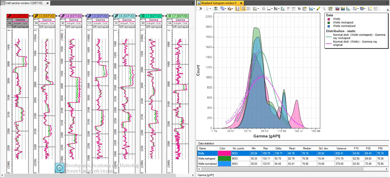 {width="6.197916666666667in" height="2.8333333333333335in"}]
[Data reshaper tool dialog]{.underline}
[
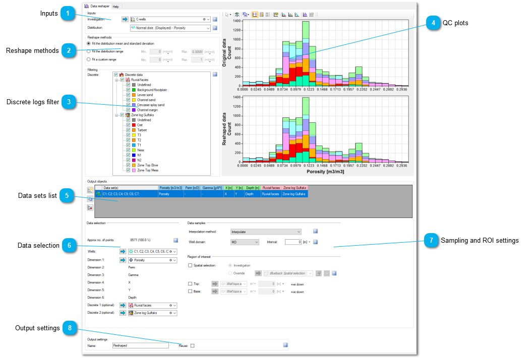 {width="6.197916666666667in" height="4.21875in"}]
[
{width="0.4166666666666667in" height="0.4166666666666667in"}]{.underline}[ Inputs]{.underline}[
 {width="5.125in" height="0.9375in"}]
[Select an investigation that contains the distribution that you would like to use for the reshaping. Then select the distribution you would like to have as the target distribution.]
[
{width="0.4166666666666667in" height="0.4166666666666667in"}]{.underline}[Reshape methods]{.underline}[
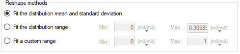 {width="5.09375in" height="1.1666666666666667in"}]
[Choose the method of reshaping.]
[The reshaping can be done in three different ways:]
[1. Fit to a distribution. The data is shifted, squeezed or stretched so that the resulting data matches a given distribution. The target distribution must be either]
[A ]{.underline}[normal distribution]{.underline}[, in which case the resulting data will have a mean and standard deviation that matches the target distribution.]
[A ]{.underline}[log normal distribution]{.underline}[, in which case the resulting data will have the same mean and standard deviation for the data's logarithm (µ σ as the target distribution.]
[2. Fit to a distribution range. The data is squeezed or stretched to match the min/max range of a Investigator distribution object.The min/max range of the data is shown in the number boxes.]
[
 {width="4.895833333333333in" height="0.34375in"}]
[3. Fit to a custom distribution. The data is squeezed or stretched to match a min/max range given by the user. The min and max values can be entered directly into the min/max number boxes.]
[
 {width="4.854166666666667in" height="0.28125in"}]
[
{width="0.4166666666666667in" height="0.4166666666666667in"}]{.underline}[Discrete logs filter]{.underline}[
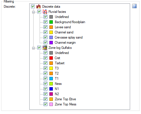 {width="5.114583333333333in" height="4.15625in"}]
[If the selected investigation has discrete dimensions, these will be available to use as filters. Please note that a filter will be ignored if no discrete log is selected in the data selection, see below in "Data selection".]
[Only data that matches the filter selection will be used for reshaping, and only this data will be output in the final result. A change in the filtering is reflected in the QC plot right away.]
[
{width="0.4166666666666667in" height="0.4166666666666667in"}]{.underline}[QC plots]{.underline}[
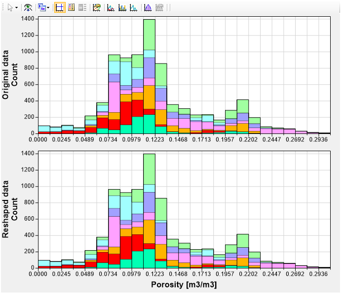 {width="6.197916666666667in" height="5.322916666666667in"}]
[Based on the current log selection and filter status, the QC plot will always show the current input data in the upper plot and the reshaped result in the lower plot. ]
[The plot functionality is a subset of the main Investigator histogram plot functionality. Please refer to Histogram]{.underline} and [Histogram toolbar]{.underline} for more information.
[Use the buttons above the plot ]
[The legend toggle button and the statistics toggle button can be used to show the legend and/or statistics. ]
[
 {width="3.78125in" height="0.3125in"}]
[If the legend is turned on, the reshaped wells are denoted with a "(r)" postfix in their name.]
[
 {width="0.8125in" height="1.0208333333333333in"}]
[Example statistics (per well):]
[
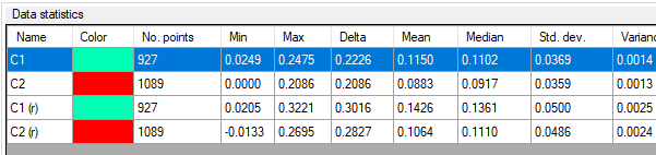 {width="6.197916666666667in" height="1.4583333333333333in"}]
[Tip:]{.underline}[ If you want to see the aggregated statistics for all wells, right click on the bars in the plot (or in the legend) and toggle the "Color by wells" option. You need to do this both for the upper and lower plot. ]
[Example aggregated statistics:]
[
 {width="6.197916666666667in" height="1.1770833333333333in"}]
[
{width="0.4166666666666667in" height="0.4166666666666667in"}]{.underline}[Data sets list]{.underline}[
 {width="6.197916666666667in" height="0.7916666666666666in"}]
[Create a new dataset with the "Add dataset" button to get started:
 {width="0.2708333333333333in" height="0.3020833333333333in"}]
[Selections of wells and logs can now be done directly in the list, but this will be the same selections as can be done as described under "Data selection".]
[Use the remove dataset button
 {width="0.3229166666666667in" height="0.3020833333333333in"} to delete a dataset and the copy dataset button
  {width="0.3125in" height="0.3125in"} to duplicate the selected dataset.]
[The list allows addition of several datasets, all with their own well and log selections. This way, several well and log combinations can be reshaped at the same time.]
[Note:]{.underline}[ Be aware however, that one output log will be created for each well per dataset. The reshaping is done sequentially dataset by dataset. Hence, if the same well is selected in more than one dataset, the output log from the subsequent datasets will have another name, ie. a postfix, to separate it from the results from the previous dataset(s). Take care to avoid confusion.]
[
{width="0.4166666666666667in" height="0.4166666666666667in"}]{.underline}[Data selection]{.underline}[
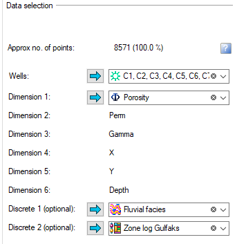 {width="3.7083333333333335in" height="3.6770833333333335in"}]
[Select the data that is to be reshaped, ie. wells and a well log. Note that all dimensions are listed, but only the well log for the dimension to be reshaped can be selected. ]
[If the filter option is to be used, discrete logs must also be selected. This is optional and the filtering will be ignored if no discrete well log was selected. ]
[
{width="0.4166666666666667in" height="0.4166666666666667in"}]{.underline}[Sampling and ROI settings]{.underline}[
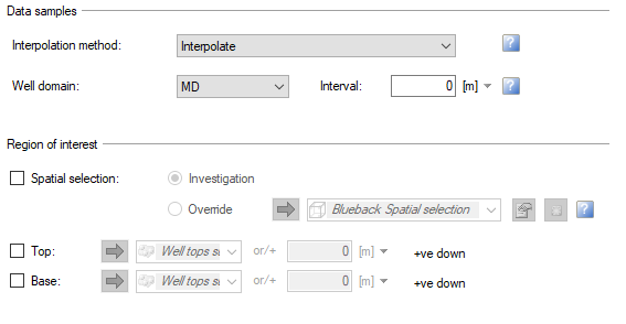 {width="5.90625in" height="3.0625in"}]
[These selections are used to choose how the well logs are sampled as well as to limit the region of interest of the data. These options are the same as in the main investigation setup dialog described here Data selection]{.underline}.
[The region of interest can be defined by either using a Blueback spatial selection object, or by selection top or base surfaces or values. The data limitation will be reflected in the QC plots.]
[
{width="0.4166666666666667in" height="0.4166666666666667in"}]{.underline}[Output settings]{.underline}[
 {width="6.197916666666667in" height="0.4479166666666667in"}]
[Set the name of the output log. Check the "Reuse" box to try to overwrite the previously created log, if possible.]
[Note:]{.underline}[ Be aware that output logs may get numerals as postfix if the previous log could not be overwritten, or if several datasets are defined.]
[Discrete template generator tool]{.underline}
[Petrel has no concept of a discrete seismic volume. Some QI workflows produces discrete classified seismic volumes. This is most often done by using a normal seismic volume and populate it with values in specific parts of the value range. This tool is created to help facilitate this specific problem but can be used to create templates from text files and edit existing templates.]
[
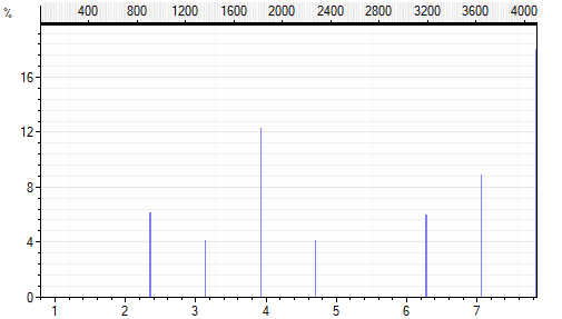 {width="5.260416666666667in" height="2.9895833333333335in"}]
[Discrete seismic value range histogram]{.underline}
[To be able to load this data into Investigator as a "discrete seismic volume" we need to create a template that has the correct number of entries, in the correct order so we can map this up in Investigator. The discrete template generator tool will analyze the seismic data and create a color table that the user can edit:]
[
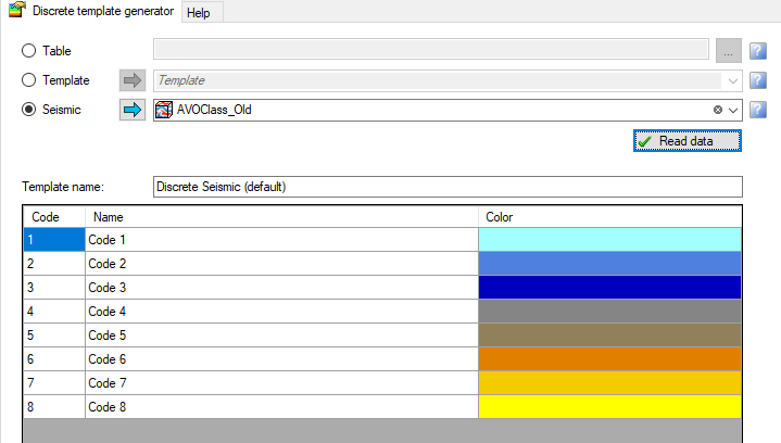 {width="6.197916666666667in" height="3.5104166666666665in"}]
[The template will be saved under Templates- Color tables/Discrete color tables:]
[
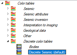 {width="2.65625in" height="1.8958333333333333in"}]
[Setting up an investigation with discrete seismic]{.underline}
[AVO Example: Intercept and gradient colored with AVO class]
[
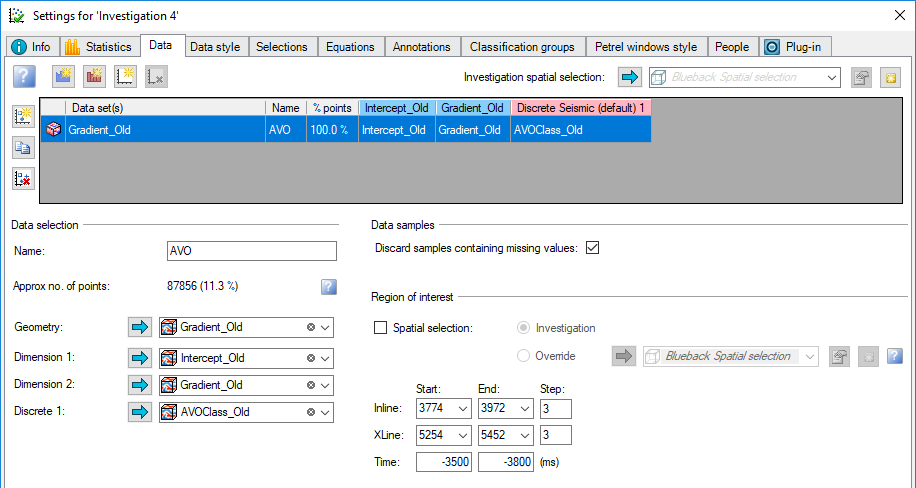 {width="6.197916666666667in" height="3.2916666666666665in"}]
[
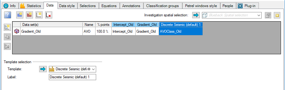 {width="6.197916666666667in" height="1.96875in"}]
[Import the Intercept and Gradient volumes as continuous dimensions. Attach the AVO volume as a discrete volume and locate the template generated by the tool. Use this template as input to the Template selection.]
[Now you can color the crossplot with the AVO discrete data:]
[
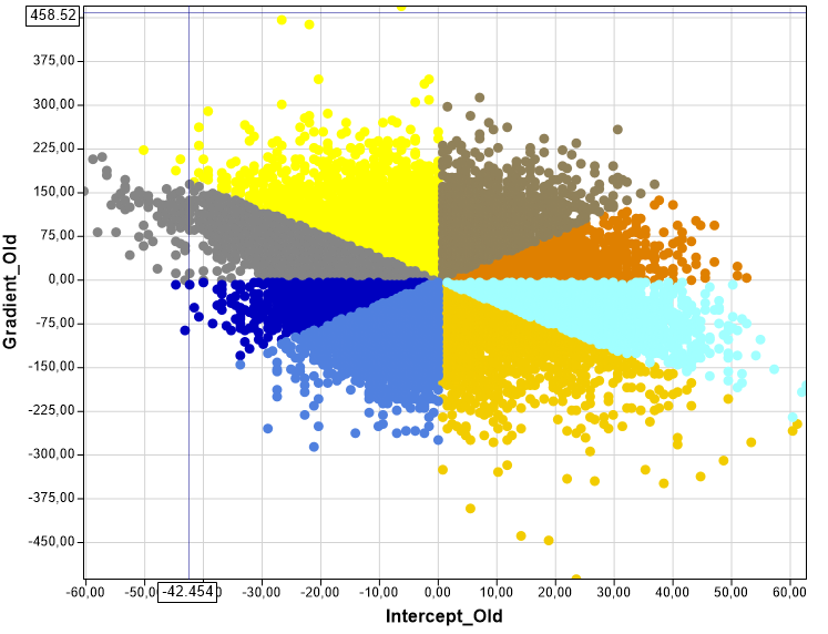 {width="6.197916666666667in" height="4.739583333333333in"}]
[Create template from Table data]
[User wants to load the information in the following as a discrete template:]
[
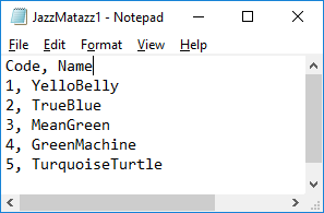 {width="3.09375in" height="2.03125in"}]
[Open tool and select the table option. Locate the text file and press read data. The Import table dialog pops up:]
[
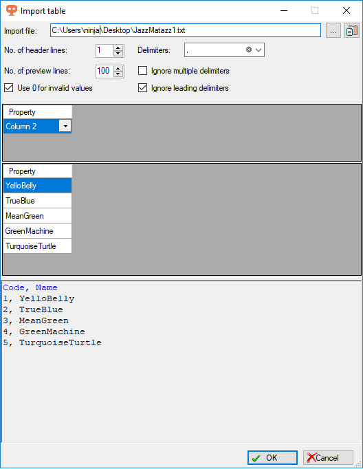 {width="5.5in" height="7.104166666666667in"}]
[Press OK, and adjust the colors as you see fit. Press apply to save the template to the template data selection pane.]
[
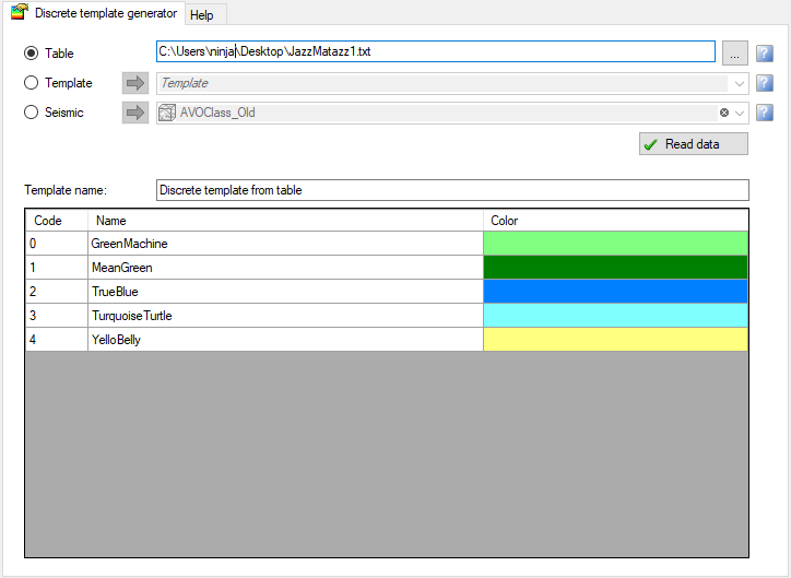 {width="6.197916666666667in" height="4.520833333333333in"}]
[Discrete template generator tool dialog]{.underline}
[
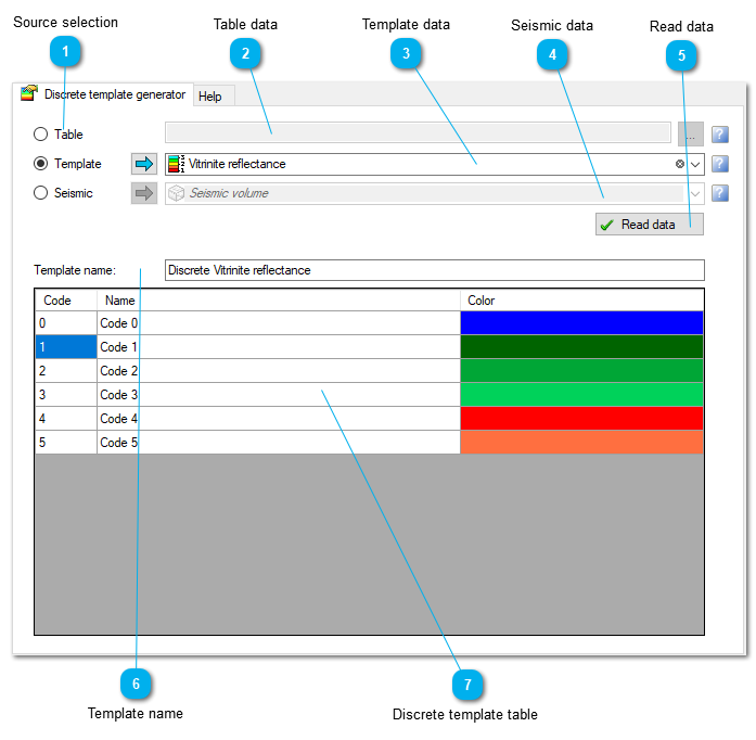 {width="6.197916666666667in" height="6.0625in"}]
[
{width="0.4166666666666667in" height="0.4166666666666667in"}]{.underline}[Source selection]{.underline}[
 {width="6.197916666666667in" height="0.7708333333333334in"}]
[Use the toggles to select the type of data to be used as source for the discrete template.]
[Use Table to import data from a text file]
[Use Template to use a continuous template]
[Use seismic to use seismic data ]
[
{width="0.4166666666666667in" height="0.4166666666666667in"}]{.underline}[Table data]{.underline}[
 {width="6.197916666666667in" height="0.2708333333333333in"}]
[Select Table toggle and the text file to be read. When Read data is clicked, a new dialog will open.]
[In this new dialog, choose the header lines, delimiters and the column of the data to be used.]
[Random colors will be assigned to the new template.]
[
{width="0.4166666666666667in" height="0.4166666666666667in"}]{.underline}[Template data]{.underline}[
 {width="6.197916666666667in" height="0.2708333333333333in"}]
[Select Template toggle and use the drop down box to select the continuous template to be used. These templates are already filtered, the ones shown have discontinuities.]
[When Read data is clicked, the discontinuities will be detected and used as input for the new template. ]
[The template colors will be used.]
[
{width="0.4166666666666667in" height="0.4166666666666667in"}]{.underline}[Seismic data]{.underline}[
 {width="6.197916666666667in" height="0.2708333333333333in"}]
[Select Seismic toggle and use the drop down box to select the desired seismic cube to be used as input. ]
[Any seismic can be used but it works better with seismic that is suitable for discretization.]
[When Read data is clicked, the cube will be read and all values will be discretized, creating the items of the template. ]
[The original color from the seismic will be used.]
[
{width="0.4166666666666667in" height="0.4166666666666667in"}]{.underline}[Read data]{.underline}[
 {width="1.1458333333333333in" height="0.2916666666666667in"}]
[When clicked, the discrete template table will be populated with the data read from the selected source.]
[
{width="0.4166666666666667in" height="0.4166666666666667in"}]{.underline}[Template name]{.underline}[
 {width="6.197916666666667in" height="0.2916666666666667in"}]
[Choose a name for the template to be created.]
[
{width="0.4166666666666667in" height="0.4166666666666667in"}]{.underline}[Discrete template table ]{.underline}[
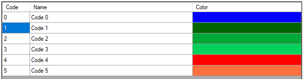 {width="6.197916666666667in" height="1.6041666666666667in"}]
[Here, the names and colors can be edited before clicking apply to create the template.]
[Worksteps]{.underline}
[Blueback Investigator supports basic worksteps to allow creation, population and display of an investigation.]
[Due to the way workflows are processed in Petrel it is not possible to perform creation and population of an investigation within the workflow.]
[An investigation creation workflow can contain the create investigation]{.underline} and [add dimension]{.underline} worksteps.
[A populate investigation workflow can contain add dataset]{.underline} and optionally one or more of the following worksteps:
[Create investigation workstep]{.underline}
[This workstep creates a new empty investigation in the Petrel input tree.]
[
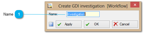 {width="5.166666666666667in" height="1.2291666666666667in"}]
[
{width="0.4166666666666667in" height="0.4166666666666667in"}]{.underline}[Name]{.underline}[
 {width="1.8854166666666667in" height="0.2708333333333333in"}]
[The name of the new investigation]
[Add dimension workstep]{.underline}
[This workstep adds a new ]{.underline}[dimension]{.underline}[ to the selected investigation.]
[
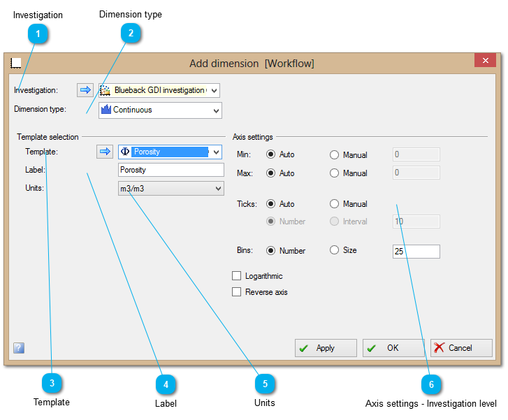 {width="6.197916666666667in" height="5.114583333333333in"}]
[
{width="0.4166666666666667in" height="0.4166666666666667in"}]{.underline}[Investigation]{.underline}[
 {width="3.1979166666666665in" height="0.3854166666666667in"}]
[Selects the dimension to which the dimension will be added.]
[
{width="0.4166666666666667in" height="0.4166666666666667in"}]{.underline}[Dimension type]{.underline}[
 {width="3.1979166666666665in" height="0.3229166666666667in"}]
[Controls the type of dimension to be added.]
[
{width="0.4166666666666667in" height="0.4166666666666667in"}]{.underline}[Template]{.underline}[
 {width="3.1354166666666665in" height="0.34375in"}]
[Controls the selected template for the dimension]
[
{width="0.4166666666666667in" height="0.4166666666666667in"}]{.underline}[Label]{.underline}[
 {width="3.0729166666666665in" height="0.2916666666666667in"}]
[Set display name of the dimension. The label name will be used in all the plots. Default is to have the same label name as the Template name.]
[
{width="0.4166666666666667in" height="0.4166666666666667in"}]{.underline}[Units]{.underline}[
 {width="3.0729166666666665in" height="0.2916666666666667in"}]
[Set the display units for the dimension.]
[
{width="0.4166666666666667in" height="0.4166666666666667in"}]{.underline}[Axis settings - Investigation level]{.underline}[
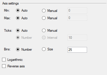 {width="3.90625in" height="2.7604166666666665in"}]
[Controls the Investigation level axis settings for windows. See Axis settings]{.underline} for more information
[Add dataset workstep]{.underline}
[This workstep add a new ]{.underline}[dataset]{.underline}[ to the selected investigation.]
[
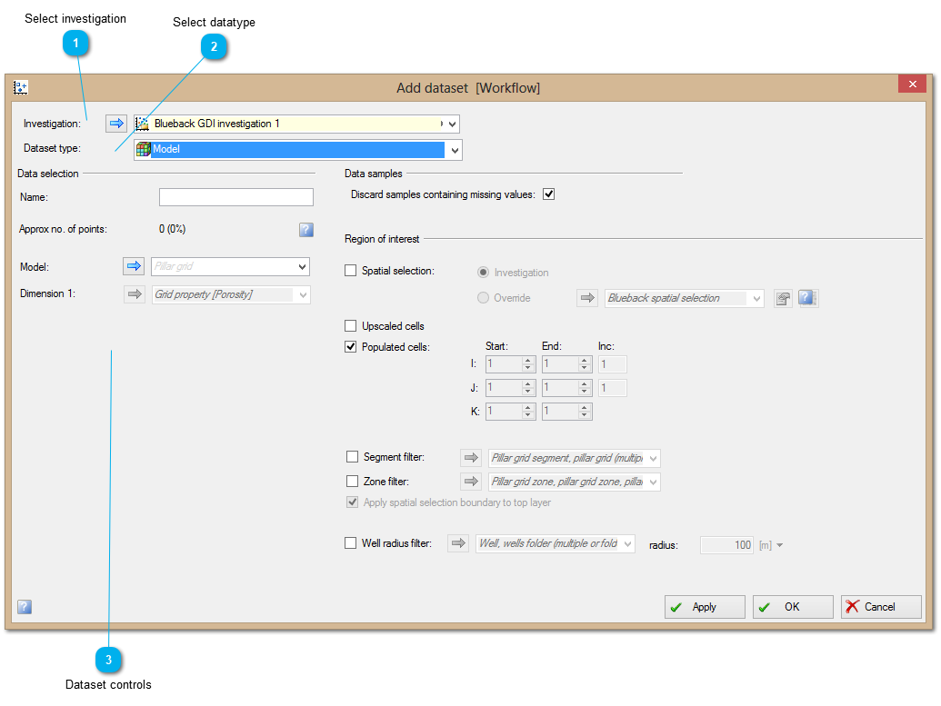 {width="6.197916666666667in" height="4.645833333333333in"}]
[
{width="0.4166666666666667in" height="0.4166666666666667in"}]{.underline}[Select investigation]{.underline}[
 {width="5.114583333333333in" height="0.2916666666666667in"}]
[Select the investigation to which the dataset will be added.]
[
{width="0.4166666666666667in" height="0.4166666666666667in"}]{.underline}[Select datatype]{.underline}[
 {width="5.15625in" height="0.2916666666666667in"}]
[Select the datatype to be added to the investiation.]
[
{width="0.4166666666666667in" height="0.4166666666666667in"}]{.underline}[Dataset controls]{.underline}[The dataset controls will be displayed here based on the selected datatype.]
[For specific dataset control information see datasets]
[Open histogram window workstep]{.underline}
[This workstep displays the selected investigation in a new histogram window. ]
[
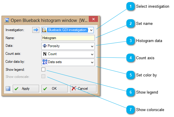 {width="6.125in" height="4.114583333333333in"}]
[
{width="0.4166666666666667in" height="0.4166666666666667in"}]{.underline}[Select investigation]{.underline}[
 {width="3.1875in" height="0.3020833333333333in"}]
[Select the investigation to be displayed]
[
{width="0.4166666666666667in" height="0.4166666666666667in"}]{.underline}[Set name]{.underline}[
 {width="3.2291666666666665in" height="0.3125in"}]
[The name to be given to the opened window]
[
{width="0.4166666666666667in" height="0.4166666666666667in"}]{.underline}[Histogram data]{.underline}[
 {width="3.21875in" height="0.3229166666666667in"}]
[Select the dimension data to show in the histogram]
[
{width="0.4166666666666667in" height="0.4166666666666667in"}]{.underline}[Count axis]{.underline}[
 {width="3.2083333333333335in" height="0.2916666666666667in"}]
[Select the count axis type to be shown]
[
{width="0.4166666666666667in" height="0.4166666666666667in"}]{.underline}[Set color by]{.underline}[
 {width="3.1979166666666665in" height="0.3020833333333333in"}]
[Select how the data should be colored]
[
{width="0.4166666666666667in" height="0.4166666666666667in"}]{.underline}[Show legend]{.underline}[
 {width="1.4895833333333333in" height="0.25in"}]
[Select whether the legend should be displayed or not]
[
{width="0.4166666666666667in" height="0.4166666666666667in"}]{.underline}[Show colorscale]{.underline}[
 {width="1.4479166666666667in" height="0.2916666666666667in"}]
[If the data is colored by a continuous dimension then should the colorscale be shown]
[Open crossplot window workstep]{.underline}
[This workstep displays the selected investigation in a new crossplot window. ]
[
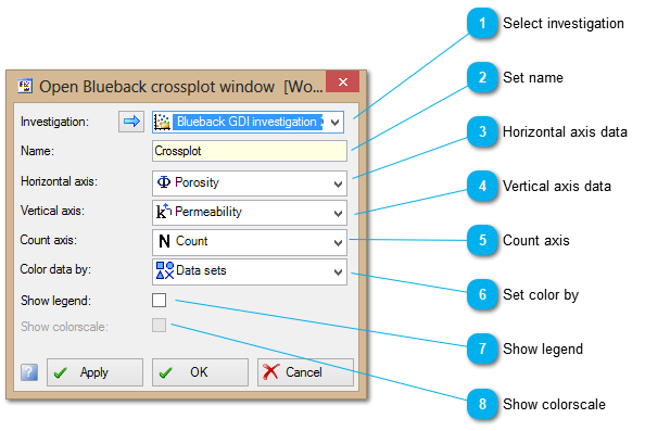 {width="6.1875in" height="4.135416666666667in"}]
[
{width="0.4166666666666667in" height="0.4166666666666667in"}]{.underline}[Select investigation]{.underline}[
 {width="3.1875in" height="0.3020833333333333in"}]
[Select the investigation to be displayed]
[
{width="0.4166666666666667in" height="0.4166666666666667in"}]{.underline}[Set name]{.underline}[
 {width="3.2291666666666665in" height="0.3125in"}]
[The name to be given to the opened window]
[
{width="0.4166666666666667in" height="0.4166666666666667in"}]{.underline}[Horizontal axis data]{.underline}[
 {width="3.21875in" height="0.3229166666666667in"}]
[Select the dimension data to be shown on the horizontal axis]
[
{width="0.4166666666666667in" height="0.4166666666666667in"}]{.underline}[Vertical axis data]{.underline}[
 {width="3.1979166666666665in" height="0.2916666666666667in"}]
[Select the dimension data to be shown on the vertical axis]
[
{width="0.4166666666666667in" height="0.4166666666666667in"}]{.underline}[Count axis]{.underline}[
 {width="3.2083333333333335in" height="0.2916666666666667in"}]
[Select the count axis type to be shown on the histograms]
[
{width="0.4166666666666667in" height="0.4166666666666667in"}]{.underline}[Set color by]{.underline}[
 {width="3.1979166666666665in" height="0.3020833333333333in"}]
[Select how the data should be colored]
[
{width="0.4166666666666667in" height="0.4166666666666667in"}]{.underline}[Show legend]{.underline}[
 {width="1.4895833333333333in" height="0.25in"}]
[Select whether the legend should be displayed or not]
[
{width="0.4166666666666667in" height="0.4166666666666667in"}]{.underline}[Show colorscale]{.underline}[
 {width="1.4479166666666667in" height="0.2916666666666667in"}]
[If the data is colored by a continuous dimension then should the colorscale be shown]
[Open matrix window workstep]{.underline}
[This workstep displays the selected investigation in a new matrix window. ]
[
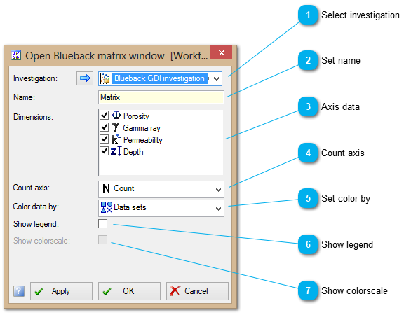 {width="6.104166666666667in" height="4.6875in"}]
[
{width="0.4166666666666667in" height="0.4166666666666667in"}]{.underline}[Select investigation]{.underline}[
{width="3.1875in" height="0.3020833333333333in"}][Select the investigation to be displayed]
[
{width="0.4166666666666667in" height="0.4166666666666667in"}]{.underline}[Set name]{.underline}[
 {width="3.2291666666666665in" height="0.3125in"}]
[The name to be given to the opened window]
[
{width="0.4166666666666667in" height="0.4166666666666667in"}]{.underline}[Axis data]{.underline}[
 {width="3.21875in" height="1.0833333333333333in"}]
[Select the dimensions to be shown in the matrix window]
[
{width="0.4166666666666667in" height="0.4166666666666667in"}]{.underline}[Count axis]{.underline}[
 {width="3.2083333333333335in" height="0.2916666666666667in"}]
[Select the count axis type to be shown on the histograms]
[
{width="0.4166666666666667in" height="0.4166666666666667in"}]{.underline}[Set color by]{.underline}[
 {width="3.1979166666666665in" height="0.3020833333333333in"}]
[Select how the data should be colored]
[
{width="0.4166666666666667in" height="0.4166666666666667in"}]{.underline}[Show legend]{.underline}[
 {width="1.4895833333333333in" height="0.25in"}]
[Select whether the legend should be displayed or not]
[
{width="0.4166666666666667in" height="0.4166666666666667in"}]{.underline}[Show colorscale]{.underline}[
 {width="1.4479166666666667in" height="0.2916666666666667in"}]
[If the data is colored by a continuous dimension then should the colorscale be shown]
[Open parallel coordinates window workstep]{.underline}
[This workstep displays the selected investigation in a new parallel coordinates window. ]
[
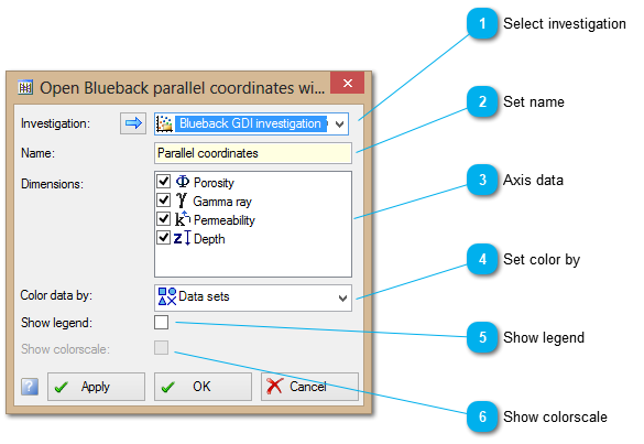 {width="6.09375in" height="4.197916666666667in"}]
[
{width="0.4166666666666667in" height="0.4166666666666667in"}]{.underline}[Select investigation]{.underline}[
{width="3.1875in" height="0.3020833333333333in"}][Select the investigation to be displayed]
[
{width="0.4166666666666667in" height="0.4166666666666667in"}]{.underline}[Set name]{.underline}[
 {width="3.2291666666666665in" height="0.3125in"}]
[The name to be given to the opened window]
[
{width="0.4166666666666667in" height="0.4166666666666667in"}]{.underline}[Axis data]{.underline}[
 {width="3.21875in" height="1.0833333333333333in"}]
[Select the dimensions to be shown in the window]
[
{width="0.4166666666666667in" height="0.4166666666666667in"}]{.underline}[Set color by]{.underline}[
 {width="3.1979166666666665in" height="0.3020833333333333in"}]
[Select how the data should be colored.]
[
{width="0.4166666666666667in" height="0.4166666666666667in"}]{.underline}[Show legend]{.underline}[
 {width="1.4895833333333333in" height="0.25in"}]
[Select whether the legend should be displayed or not]
[
{width="0.4166666666666667in" height="0.4166666666666667in"}]{.underline}[Show colorscale]{.underline}[
 {width="1.4479166666666667in" height="0.2916666666666667in"}]
[If the data is colored by a continuous dimension then should the colorscale be shown]
[Blueback Spatial Selector]{.underline}
[Blueback Spatial Selector is a free Blueback software product which allows the user to define and manipulate regions of interest interactively within the majority of Petrel windows. These spatial selections can be used in Blueback products when required. ]
[The Blueback Spatial Selector aims to ensure more repeatable/error free workflows by providing a quick and easy way for users to constrain data to specifically defined spatial regions.]
[The spatial selection allows the user to define a region of interest in X/Y/Z space and optionally top and base surfaces and a boundary polygon.]
[Please see the Blueback Spatial Selector user guide for more information.]
[Using spatial selections within Blueback Investigator]{.underline}
[Blueback spatial selections can be used within Blueback Investigator in the following ways:]
[Define the region of interest to be investigated (see Investigation spatial selection]{.underline})
[Create a new investigation from the selected Petrel objects (see Create investigation from spatial selection]{.underline})
[A spatial filter can be used to help identify points of interest within an investigation (see Blueback Spatial selections as filters]{.underline})
[Create investigation from spatial selection]{.underline}
[From the ]{.underline}[spatial selection]{.underline}[ context menu select the ]{.underline}[Create investigation...]{.underline}[ option. This provides a quick and easy way to start investigating the domain object displayed in the currently selected Petrel window.]
[The data selection]{.underline} dialog will be opened and will be pre-populated with datasets for the currently visible objects.
[
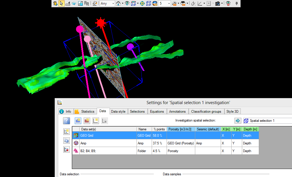 {width="6.197916666666667in" height="3.7604166666666665in"}]
[The investigation can be changed as necessary to add/remove ]{.underline}[dimensions]{.underline}[ and ]{.underline}[datasets]{.underline}[.]
[Blueback Spatial selections as filters]{.underline}
[Blueback spatial selections can be used within Blueback Investigator as a spatial filter. This can be useful to determine which points within the investigation relate to a feature identified in a Petrel window.]
[Note: The investigation must contain spatial dimensions.]{.underline}
[With a Blueback Investigator window active, the user can toggle to display a Blueback Spatial Selection in the Petrel tree.]
[
 {width="2.5625in" height="0.53125in"}]
[The displayed points in the Blueback window will than update to use the Blueback Spatial Selection as a filter. Moving the Blueback Spatial Selection will interactively update the points in the Blueback Investigator window to show which points are filtered and which are not.]
[
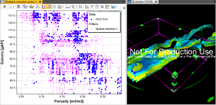 {width="6.197916666666667in" height="3.03125in"}]
[Prizm Investigator]{.underline}
[Prizm Investigator allows a user to connect from Python to a running Blueback Investigator providing access to investigations and the ability to plot investigation data from Python.]
[Prizm Investigator as an evolution of InvestigatorPy. The InvestigatorPy implementation was found by users to be very restrictive due to the need for very specific setup, only available on Windows and requiring a specific Python version. Prizm Investigator provides support for more flexible deployment scenarios and removes the restriction on Python version. ]
[Detailed documentation about Prizm Investigator can be found here]{.underline}. The online documentation contains installation information along with API documentation, user guides and example workflows. The online documentation will be continually updated and improved based on user feedback/questions.
[Data transfer between Petrel and Python]{.underline}
[The original InvestigatorPy functionality supports transfer of data between Petrel and Python via file. An .invpy file]{.underline} can be exported from Petrel and loaded in Python. [Predictors]{.underline} and [classifiers]{.underline} can be created in Python and imported in Petrel.
[Prizm Investigator supports seamless data transfer between Petrel and Python. This is facilitated by Cegal Hub, allowing electronic data transfer without the need for manual files. Example notebooks showing the use of predictors and classifiers in Python and transferring to Petrel can be here]{.underline}.
[InvestigatorPy]{.underline}
[The InvestigatorPy package has been retired.]
[All users must convert existing Python code to use Prizm Investigator. ]
[Python Setup]{.underline}
[The python for using Prizm Investigator can be setup in many different ways depending on various factors. ]
[ ]
[Example deployments may include:]
[an open cloud environment]
[an IT controlled locked down python environment running on a company data center]
[an IT provided local python environment on the users machine]
[an minimal managed Prizm environment provided by the Blueback Investigator plugin]
[See the Installation Guide for Blueback Investigator for full details of how to setup an usable Python environment.]
[Blueback Investigator installer includes all the files necessary to deploy and configure a minimal managed Prizm environment on the users local PC (see Prizm Environments for Investigator]{.underline})
[Prizm Environments for Investigator]{.underline}
[Prizm Environments is a utility for deploying and managing Python environments required to run Prizm workflows in Petrel. It allows you to set up these environments and their associated workflows directly on your computer. For more information, please navigate to the online documentation (Cegal Prizm documentation]{.underline}).
[
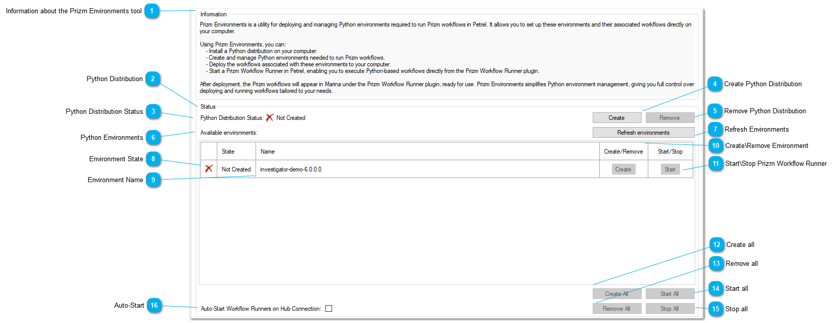 {width="6.197916666666667in" height="2.3958333333333335in"}]
[
{width="0.4166666666666667in" height="0.4166666666666667in"}]{.underline}[Information about the Prizm Environments tool]{.underline}[
 {width="6.197916666666667in" height="1.125in"}]
[This section provides an overview of Prizm Environments, explaining its purpose, how it manages Python environments, and how it integrates with the Prizm Workflow Runner in Petrel.]
[Depending on IT configuration, this section may look different. If IT has restricted the tool, all functionality will be disabled. If IT has automated deployment, users will only be able to start and stop Prizm Workflow Runners. In both cases, the following message will be displayed:]
["The configuration of the Prizm Environments tool has been restricted by your IT department.]
[Please contact your IT administrator if you need further information or assistance."]
[
{width="0.4166666666666667in" height="0.4166666666666667in"}]{.underline}[Python Distribution]{.underline}[
 {width="6.197916666666667in" height="0.2708333333333333in"}]
[A Python distribution is required to create and manage Python environments. This section displays the current status of the Python distribution and allows users to install or remove it using the Create and Remove buttons.]
[
{width="0.4166666666666667in" height="0.4166666666666667in"}]{.underline}[Python Distribution Status]{.underline}[
 {width="2.3125in" height="0.2916666666666667in"}]
[Indicates the current state of the Python distribution:]
[Not Created --The Python distribution is not installed.]
[In Progress --The Python distribution is being installed or removed.]
[Available --The Python distribution is installed and ready for use.]
[
{width="0.4166666666666667in" height="0.4166666666666667in"}]{.underline}[Create Python Distribution]{.underline}[
 {width="1.1145833333333333in" height="0.2916666666666667in"}]
[Clicking Create will install the required Python distribution on the user' computer. This step is necessary before Python environments can be created.]
[
{width="0.4166666666666667in" height="0.4166666666666667in"}]{.underline}[Remove Python Distribution]{.underline}[
 {width="1.0520833333333333in" height="0.3229166666666667in"}]
[Clicking Remove will uninstall the Python distribution.]
[Note]{.underline}[: You must remove all environments created with this Python distribution before uninstalling it. Environments may still exist even if they are not listed in the Prizm Environments tool.]
[If the removal fails due to an existing environment, a message will appear in the Petrel message log, specifying which environment is preventing the uninstallation:]
[Prizm Environments[Investigator]: Remaining environment(s) found (<EnvironmentName>). Python distribution was not uninstalled.]{.underline}
[
{width="0.4166666666666667in" height="0.4166666666666667in"}]{.underline}[Python Environments]{.underline}[
 {width="6.197916666666667in" height="0.6770833333333334in"}]
[This section displays a list of all available Python environments and their current status. Users can create or remove environments and start or stop the associated Prizm Workflow Runners.]
[
{width="0.4166666666666667in" height="0.4166666666666667in"}]{.underline}[Refresh Environments]{.underline}[
 {width="2.1354166666666665in" height="0.2916666666666667in"}]
[Clicking Refresh Environments updates the list of environments to reflect any changes, such as newly created or removed environments.]
[
{width="0.4166666666666667in" height="0.4166666666666667in"}]{.underline}[Environment State]{.underline}[
 {width="1.1875in" height="0.8645833333333334in"}]
[Indicates the status of each Python environment:]
[Not Created --The environment has not been set up yet.]
[Initialising --The environment is being created.]
[Available --The environment is ready for use, and a Prizm Workflow Runner can be started.]
[Removing --The environment is being removed.]
[Running --The Prizm Workflow Runner associated with the environment is running.]
[Error --An issue occurred during environment creation, removal, or when starting a Prizm Workflow Runner. Check the Petrel message log for more details.]
[
{width="0.4166666666666667in" height="0.4166666666666667in"}]{.underline}[Environment Name]{.underline}[
 {width="1.5520833333333333in" height="0.7604166666666666in"}]
[Displays the name of each environment.]
[
{width="0.4166666666666667in" height="0.4166666666666667in"}]{.underline}[Create]{.underline}[\]{.underline}[Remove Environment]{.underline}[
 {width="1.0104166666666667in" height="0.7708333333333334in"}]
[Create]{.underline}[ --Sets up a new Python environment and deploys the associated Prizm workflows. A Python distribution must be available before creating an environment.]
[Remove]{.underline}[ --Deletes the environment from the machine. A running Prizm Workflow Runner must be stopped before removing an environment.]
[
{width="0.4166666666666667in" height="0.4166666666666667in"}]{.underline}[Start]{.underline}[\]{.underline}[Stop Prizm Workflow Runner]{.underline}[
 {width="0.9583333333333334in" height="0.7916666666666666in"}]
[Start]{.underline}[ --Launches a Prizm Workflow Runner within the selected Python environment. Once started, users can access the associated Prizm workflows in the Prizm Workflow Runner plugin.]
[Stop]{.underline}[ --Shuts down the Prizm Workflow Runner for the selected environment. Once stopped, Prizm workflows will no longer be accessible in the Prizm Workflow Runner plugin.]
[Note]{.underline}[: The associated Python environment must be created before starting or stopping the Prizm Workflow Runner.]
[
{width="0.4166666666666667in" height="0.4166666666666667in"}]{.underline}[Create all]{.underline}[
 {width="1.0625in" height="0.2916666666666667in"}]
[Clicking Create All will set up all available environments.]
[Note]{.underline}[: A Python distribution must be created before creating environments.]
[
{width="0.4166666666666667in" height="0.4166666666666667in"}]{.underline}[Remove all]{.underline}[
 {width="1.09375in" height="0.2916666666666667in"}]
[Deletes all Cegal-managed environments created through Prizm Environments.]
[Note]{.underline}[: This does not affect manually created environments. Any running Prizm Workflow Runners must be stopped before removing environments.]
[
{width="0.4166666666666667in" height="0.4166666666666667in"}]{.underline}[Start all]{.underline}[
 {width="1.0625in" height="0.2916666666666667in"}]
[Launches a Prizm Workflow Runner for each available environment, making all associated Prizm workflows accessible in the Prizm Workflow Runner plugin.]
[
{width="0.4166666666666667in" height="0.4166666666666667in"}]{.underline}[Stop all]{.underline}[
 {width="1.0625in" height="0.3020833333333333in"}]
[Stops all running Prizm Workflow Runners, removing access to workflows in the Prizm Workflow Runner plugin.]
[
{width="0.4166666666666667in" height="0.4166666666666667in"}]{.underline}[Auto-Start]{.underline}[
 {width="2.8020833333333335in" height="0.2916666666666667in"}]
[Enabling this option ensures that all available Prizm Workflow Runners automatically start whenever Petrel connects to a Hub server.]
[.invpy file]{.underline}
[A .invpy file is a compressed, binary file containing the information from a Blueback Investigation. ]
[It can be exported from Petrel via the toolbar button or the investigation context menu.]
[The invpy file is accessed in the python environment using the investigatorpy package. This Python environment can be on the same PC, in a local HPC environment or in the cloud. For example, if a complex machine learning model needs to be trained then a multi-core cluster of python nodes in the cloud could be used to reduce the training time.]
[The following snippet from a jupyter notebook shows loading an invpy file into Python and the dataframe that was created.]
[
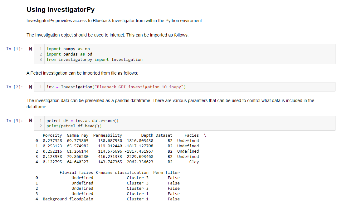 {width="6.197916666666667in" height="3.7291666666666665in"}]
[Import Python prediction equation]{.underline}
[A Python prediction equation can be used to predict a continuous value. The equation takes a number of continuous dimension inputs and predicts a new continuous dimension. This new continuous dimension will be represented in the Investigation like any other continuous dimension.]
[This equation can be defined either by saving a predictor function using Prizm Investigator or as a function in a Python script. ]
[The Python function must be decorated with either @InvestigatorPyFunction1D or @InvestigatorPyFunction2D. This is necessary to ensure that data passed from Blueback Investigator is transformed into the correct format as required by the Python function. The predictor function saved by Prizm Investigator also defines information about the required input dimensions, the units for the dimensions and a units for the output value the function will return. Blueback Investigator uses this information to ensurr that data is passed to the Python function in the correct units. The function is encoded into the json file using a python package called cloudpickle.]
[The following example shows a simple predictor being trained in python. The dataframe (df) had already been created by loading data from a Blueback Investigation invpy file.]
[
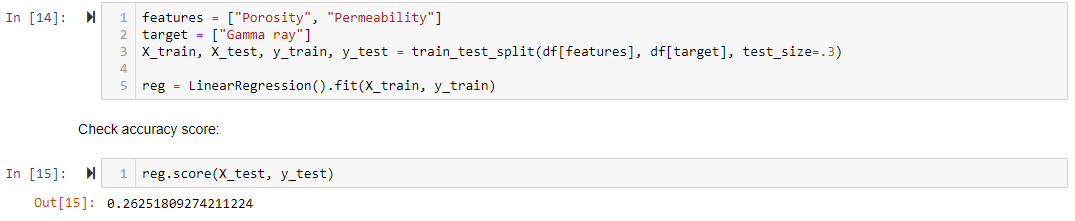 {width="6.197916666666667in" height="1.2708333333333333in"}]
[The predictor can be exported from Python as shown below. The first cell setup the necessary information that needs to be supplied with the predictor. The second cell defines the function (with the decorator) and call save_predictor. This will create a <filename>.json file to be created in the current working directly. ]
[
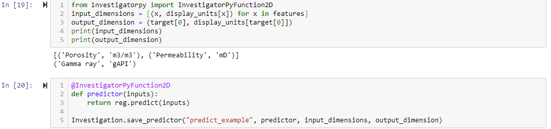 {width="6.197916666666667in" height="1.4479166666666667in"}]
[This json file can be imported into Petrel as an equation using the ]{.underline}[Add Python regression]{.underline}[ toolbar button. The input dimensions can be assigned after the json file is selected.]
[
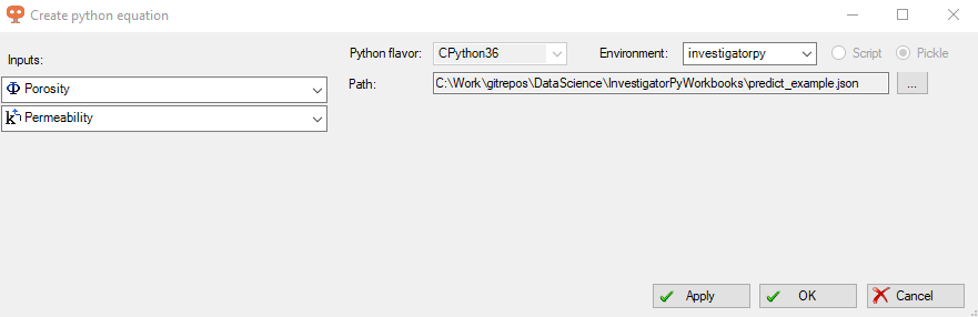 {width="6.197916666666667in" height="2.0104166666666665in"}]
[This will create a new continuous dimension in the investigation based on the information included in the json file.]
[Import Python classification equation]{.underline}
[A Python classification equation should be used to predict a discrete value. The equation takes a number of continuous dimension inputs and predicts a new discrete dimension. This new discrete dimension will be represented in the Investigation as a Classification Group.]
[This equation can be defined either by saving a classifier function using investigatorpy or as a function in a Python script. ]
[The Python function must be decorated with either @InvestigatorPyFunction1D or @InvestigatorPyFunction2D. This is necessary to ensure that data passed from Blueback Investigator is transformed into the correct format as required by the Python function. The classifier function saved by investigatorpy also contains information about the required input dimensions, the units for the dimensions and a list of output tuples the function will return. Blueback Investigator uses this information to ensure that data is passed to the Python function in the correct units and that the resulting value is assigned to the correct discrete value with the classification group. The function is encoded into the json file using a python package called cloudpickle.]
[The following example shows a simple classifier being trained in python. The dataframe (df) had already been created by loading data from a Blueback Investigation invpy file.]
[
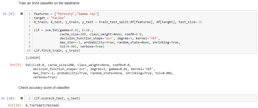 {width="6.197916666666667in" height="2.59375in"}]
[The classifier can be exported from Python as shown below. The first cell setup the necessary information that needs to be supplied with the classifier. The second cell defines the function (with the decorator) and call save_classifier. This will create a <filename>.json file to be created in the current working directly. ]
[
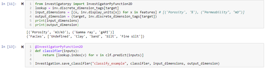 {width="6.197916666666667in" height="1.59375in"}]
[This json file can be imported into Petrel as an equation using the ]{.underline}[Add Python classification]{.underline}[ toolbar button. The input dimensions can be assigned after the json file is selected.]
[
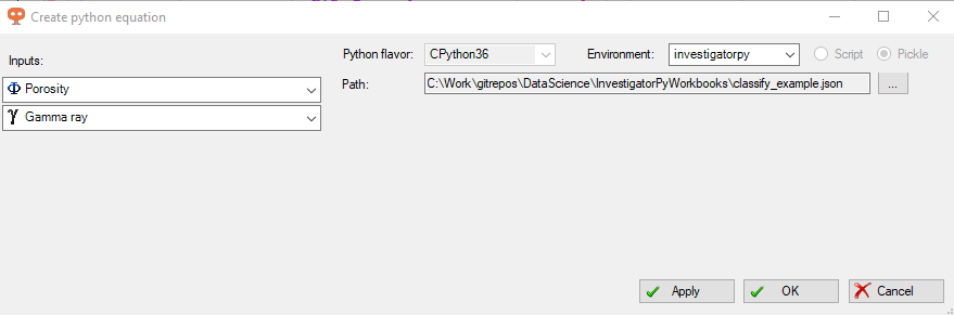 {width="6.197916666666667in" height="2.0416666666666665in"}]
[This will create a new classification group in the investigation based on the information included in the json file.]
[
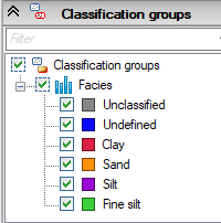 {width="2.0833333333333335in" height="2.1041666666666665in"}]
[Bundled workflows]{.underline}
[Blueback Investigator installs optional bundled workflows that allow the plugin functionality to be extended and enhanced through the use of Python. Once Prizm has been setup, these workflows can be executed directly within Petrel using the Prizm Workflow Runner]{.underline}.
[These bundled workflows serve as an example of what can be achieved using Python. Users with Python knowledge are encouraged to read and understand these workflows and customize or extend them as necessary to provide more value. If you require assistance with these workflows then please contact Cegal support who can help and provide consultants and training if necessary. ]
[Investigation Movie]{.underline}
[This workflow use seismic 3D of model properties from the selected investigation. It creates a multiple slices through each of the dimensions and stitches these images together to create a movie file showing the changing data. The direction of the movie, duration and frame rate can all be controlled by the Petrel user.]
[Model QC report]{.underline}
[This workflow creates a document comparing well logs, upscaled logs and model properties. The document will optionally contain various QC plots comparing:]
[well QC (well log v upscaled cells)]
[upscaled QC (upscaled v model cells)]
[zone maps]
[intersections]
[The selected investigation must contain well logs and a single 3D model datasets with Z spatial, facies and zone dimensions.]
[Model QC report]{.underline}
[This workflow creates a document containing a standard set of QC plots for each well. The document will optionally contain various QC plots comparing:]
[QC of all wells]
[QC per well]
[The selected investigation must contain well logs and a single 3D model datasets with Z spatial, and facies dimensions.]
[Well Production report]{.underline}
[This workflow creates a document containing a standard set of well production plots from an investigation. The document will optionally contain various QC plots comparing:]
[overall field plots]
[plots per identifier]
[general dimension plots]
[production plots]
[injection plots]
[The selected investigation must contain time series datasets for one of more identifier.]
[Petrel UX]{.underline}
[I]{.underline}[nvestigation contextual ribbon]{.underline}
[The majority of the investigation context menu options are now also available from the contextual ribbon.]
[
 {width="6.197916666666667in" height="0.5625in"}]
[Blueback Investigator tools ]{.underline}
[Access to the Blueback Investigator tools is provided via a Blueback Investigator tab group on the contextual ribbons for the custom domain objects that the tools support as inputs.]
[
 {width="6.197916666666667in" height="0.5625in"}]
[Petrel window contextual ribbon]{.underline}
[A Blueback Investigator section can be found on the contextual ribbon of the following Petrel windows:]
[3D window]
[2D window]
[Interpretation window]
[Intersection window]
[Map window]
[These commands can be used to create investigations from the currently displayed domain objects. The investigation can, optionally, be displayed in a Blueback Investigator window. ]
[
 {width="6.197916666666667in" height="0.8229166666666666in"}]
[Support]{.underline}
[For support on Cegal geoscience software products contact us on email: support.geo@cegal.com]{.underline} or visit [blueback.zendesk.com/home]{.underline}.
[Upgrade considerations]{.underline}
[V1.X to 2.X]{.underline}
[Histograms displayed as steps display as filled lines on upgrade. This is due to a design change in the software. Users need to set up the window manually to reconstruct the previous appearance.]
[V2.X to 3.X]{.underline}
[In Blueback Investigator v3.0 the histograms in the crossplot window have been made optional. Therefore the scatterplot window is now redundant and has been disabled. Any scatterplot windows in the project will remain but with limited functionality and no new scatterplot windows can be created. Users should create crossplot windows to replace the disabled scatterplot windows and remove the scatterplot windows from the project. Scatterplot windows will be removed in a future release .]
[V3.X to 4.X]{.underline}
[In Petrel 2014, seismic templates and colorscales were significantly changed. As such, investigations based on the following obsolete seismic templates will now need correcting by the user:]
[Seismic Red White Blue]
[Seismic Red White Black]
[Seismic Brown White Blue]
[Seismic Red White Blue (Transparent)]
[Seismic Black Grey White]
[V4.1 to 4.2]{.underline}
[Default numeric precision is based on the Petrel template settings.]